My watch list

Capillary surface

In fluid mechanics and mathematics, a capillary surface is a surface that represents the interface between two different fluids. As a consequence of being a surface, a capillary surface has no thickness in slight contrast with most real fluid interfaces.

Capillary surfaces are of interest in mathematics because the problems involved are very nonlinear and have interesting properties, such as discontinuous dependence on boundary data at isolated points^[1]. In particular, static capillary surfaces with gravity absent have constant mean curvature, so that a minimal surface is a special case of static capillary surface.

They are also of practical interest for fluid management in space (or other environments free of body forces), where both flow and static configuration are often dominated by capillary effects.

Additional recommended knowledge

Daily Sensitivity Test

How to quickly check pipettes?

How to ensure accurate weighing results every day?

1 The stress balance equation
- 1.1 The stress tensor
2 Static interfaces
- 2.1 Energy consideration
3 Boundary conditions
4 References

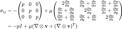
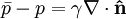
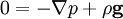
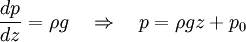
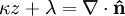
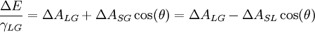
The stress balance equation

The defining equation for a capillary surface is called the stress balance equation^[2], which can be derived by considering the forces and stresses acting on a small volume that is partly bounded by a capillary surface. For a fluid meeting another fluid (the "other" fluid notated with bars) at a surface $S$ , the equation reads

$\mathbf{\hat n} \sigma_{ij} - \mathbf{\hat n} \bar{\sigma}_{ij} = \gamma \mathbf{\hat n} \nabla \cdot \mathbf{\hat n} + \nabla_S \gamma \qquad ; \quad \nabla_S \gamma = \nabla \gamma - \mathbf{\hat n} (\mathbf{\hat n} \cdot \nabla \gamma)$

where $\scriptstyle \mathbf{\hat n}$ is the unit normal pointing toward the "other" fluid (the one whose quantities are notated with bars), $\scriptstyle \sigma_{ij}$ is the stress tensor, $\scriptstyle \gamma$ is the surface tension associated with the interface, and $\scriptstyle \nabla_S$ is the surface gradient. Note that the quantity $\scriptstyle \nabla \cdot \mathbf{\hat n}$ is twice the mean curvature of the surface.

In fluid mechanics, this equation serves as a boundary condition for interfacial flows, typically complementing the Navier-Stokes equations. It describes the discontinuity in stress that is balanced by forces at the surface. As a boundary condition, it is somewhat unusual in that it introduces a new variable: the surface $S$ that defines the interface. It's not too surprising then that the stress balance equation normally mandates its own boundary conditions.

For best use, this vector equation is normally turned into 3 scalar equations via dot product with the unit normal and two selected unit tangents:

$\mathbf{\hat n} \sigma_{ij} \cdot \mathbf{\hat n} - \mathbf{\hat n} \bar{\sigma}_{ij} \cdot \mathbf{\hat n} = \gamma \nabla \cdot \mathbf{\hat n}$

$\mathbf{\hat n} \sigma_{ij} \cdot \mathbf{\hat t_1} - \mathbf{\hat n} \bar{\sigma}_{ij} \cdot \mathbf{\hat t_1} = \nabla \gamma \cdot \mathbf{\hat t_1}$

$\mathbf{\hat n} \sigma_{ij} \cdot \mathbf{\hat t_2} - \mathbf{\hat n} \bar{\sigma}_{ij} \cdot \mathbf{\hat t_2} = \nabla \gamma \cdot \mathbf{\hat t_2}$

Note that the products lacking dots are matrix products, those with dots are dot products (e.g., $\scriptstyle \mathbf{\hat n} \sigma_{ij}$ is a matrix product that produces a vector, and $\scriptstyle (\mathbf{\hat n} \sigma_{ij}) \cdot \mathbf{\hat n}$ is a dot product that produces a scalar). The first equation is called the normal stress equation, or the normal stress boundary condition. The second two equations are called tangential stress equations.

The stress tensor

The stress tensor is related to velocity and pressure. It's actual form will depend on the specific fluid being dealt with, for the common case of incompressible Newtonian flow the stress tensor is given by

$\begin{align} \sigma_{ij} &= -\begin{pmatrix} p&0&0\\ 0&p&0\\ 0&0&p \end{pmatrix} + \mu \begin{pmatrix} 2 \frac{\partial u}{\partial x} & \frac{\partial u}{\partial y} + \frac{\partial v}{\partial x} & \frac{\partial u}{\partial z} + \frac{\partial w}{\partial x} \\ \frac{\partial v}{\partial x} + \frac{\partial u}{\partial y} & 2 \frac{\partial v}{\partial y} & \frac{\partial v}{\partial z} + \frac{\partial w}{\partial y} \\ \frac{\partial w}{\partial x} + \frac{\partial u}{\partial z} & \frac{\partial w}{\partial y} + \frac{\partial v}{\partial z} & 2\frac{\partial w}{\partial z} \end{pmatrix} \\ &= -p I + \mu (\nabla \otimes \mathbf{v} + (\nabla \otimes \mathbf{v})^T) \end{align}$

where $p$ is the pressure in the fluid, $\scriptstyle \mathbf{v}$ is the velocity, and $μ$ is the viscosity. Note that the outer product generates the Jacobian of velocity with respect to space.

Static interfaces

In the absence of motion, the stress tensors yield only hydrostatic pressure so that $\scriptstyle \sigma_{ij} = -pI$ , regardless of fluid type or compressibility. Considering the normal and tangential equations,

$\bar p - p = \gamma \nabla \cdot \mathbf{\hat n}$

$0 = \nabla \gamma \cdot \mathbf{\hat t}$

The first equation establishes that curvature forces are balanced by pressure forces. The second equation implies that a static interface cannot exist in the presence of nonzero surface tension gradient.

If gravity is the only body force present, the Navier-Stokes equations simplify significantly:

$0 = -\nabla p + \rho \mathbf{g}$

If coordinates are chosen so that gravity is nonzero only in the $z$ direction, this equation degrades to a particularly simple form:

$\frac{d p}{d z} = \rho g \quad \Rightarrow \quad p = \rho g z + p_0$

where $p 0$ is an integration constant that represents some reference pressure at $z = 0$ . Substituting this into the normal stress equation yields what is known as the Young-Laplace equation:

$\bar \rho g z + \bar p_0 - (\rho g z + p_0) = \gamma \nabla \cdot \mathbf{\hat n} \quad \Rightarrow \quad \Delta \rho g z + \Delta p = \gamma \nabla \cdot \mathbf{\hat n}$

where $Δ p$ is the (constant) pressure difference across the interface, and $Δρ$ is the difference in density. Note that, since this equation defines a surface, $z$ is the $z$ coordinate of the capillary surface. This nonlinear partial differential equation when supplied with the right boundary conditions will define the static interface.

The pressure difference above is a constant, but it's value will change if the $z$ coordinate is shifted. The linear solution to pressure implies that, unless the gravity term is absent, it is always possible to define the $z$ coordinate so that $Δ p = 0$ . Nondimensionalized, the Young-Laplace equation is usually studied in the form ^[1]

$\kappa z + \lambda = \nabla \cdot \mathbf{\hat n}$

where (if gravity is in the negative $z$ direction) $κ$ is positive if the denser fluid is "inside" the interface, negative if it is "outside", and zero if there is no gravity or if there is no difference in density between the fluids.

This nonlinear equation has some rich properties, especially in terms of existence of unique solutions. For example, the nonexistence of solution to some boundary value problem implies that, physically, the problem can't be static. If a solution does exist, normally it'll exist for very specific values of $λ$ , which is representative of the pressure jump across the interface. This is interesting because there isn't another physical equation to determine the pressure difference. In a capillary tube, for example, implementing the contact angle boundary condition will yield a unique solution for exactly one value of $λ$ . Solutions often aren't unique, this implies that there are multiple static interfaces possible; while they may all solve the same boundary value problem, the minimization of energy will normally favor one. Different solutions are called configurations of the interface.

Energy consideration

A deep property of capillary surfaces is the surface energy that is imparted by surface tension:

$E_S = \gamma_S A_S\,$

where $A$ is the area of the surface being considered, and the total energy is the summation of all energies. Note that every interface imparts energy. For example, if there is two different fluids (say liquid and gas) inside a solid container with gravity and other energy potentials absent, the energy of the system is

$E = \sum \gamma_S A_S = \gamma_{LG} A_{LG} + \gamma_{SG} A_{SG} + \gamma_{SL} A_{SL}\,$

where the subscripts $L G$ , $S G$ , and $S L$ respectively indicate the liquid-gas, solid-gas, and solid-liquid interfaces. Note that inclusion of gravity would require consideration of the volume enclosed by the capillary surface and the solid walls.

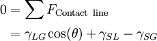
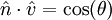
Typically the surface tension values between the solid-gas and solid-liquid interfaces are not known. This does not pose a problem; since only changes in energy are of primary interest. If the net solid area $A S G + A S L$ is a constant, and the contact angle is known, it may be shown that (again, for two different fluids in a solid container)

$E = \gamma_{SL}(A_{SL} + A_{SG}) + \gamma_{LG} A_{LG} + \gamma_{LG} A_{SG} \cos(\theta)\,$

so that

$\frac{\Delta E}{\gamma_{LG}} = \Delta A_{LG} + \Delta A_{SG} \cos(\theta) = \Delta A_{LG} - \Delta A_{SL} \cos(\theta)\,$

where $θ$ is the contact angle and the capital delta indicates the change from one configuration to another. To obtain this result, it's necessary to sum (distributed) forces at the contact line (where solid, gas, and liquid meet) in a direction tangent to the solid interface and perpendicular to the contact line:

$\begin{align} 0 &= \sum F_{\mathrm{Contact \ line}} \\ &= \gamma_{LG} \cos(\theta) + \gamma_{SL} - \gamma_{SG} \end{align}$

where the sum is zero because of the static state. When solutions to the Young-Laplace equation aren't unique, the most physically favorable solution is the one of minimum energy, though experiments (especially low gravity) show that metastable surfaces can be surprisingly persistent, and that the most stable configuration can become metastable through mechanical jarring without too much difficulty. On the other hand, a metastable surface can sometimes spontaneously achieve lower energy without any input (seemingly at least) given enough time.

Boundary conditions

Boundary conditions for stress balance describe the capillary surface at the contact line: the line where a solid meets the capillary interface; also, volume constraints can serve as boundary conditions (a suspended drop, for example, has no contact line but clearly must admit a unique solution).

For static surfaces, the most common contact line boundary condition is the implementation of the contact angle, which specifies the angle that one of the fluids meets the solid wall. The contact angle condition on the surface $S$ is normally written as:

$\hat n \cdot \hat v = \cos(\theta)\,$

where $θ$ is the contact angle. This condition is imposed on the boundary (or boundaries) $\scriptstyle \partial S$ of the surface. $\scriptstyle \hat v$ is the unit outward normal to the solid surface, and $\scriptstyle \hat n$ is a unit normal to $S$ . Choice of $\scriptstyle \hat n$ depends on which fluid the contact angle is specified for.

For dynamic interfaces, the boundary condition showed above works well if the contact line velocity is low. If the velocity is high, the contact angle will change ("dynamic contact angle"), and as of 2007 the mechanics of the moving contact line (or even the validity of the contact angle as a parameter) is not known and an area of active research^[3].

References

^ ^a ^b Robert Finn (1999). "Capillary Surface Interfaces". American Mathematical Society.
^ Surface Tension Module, by John W. M. Bush, at MIT OCW
^ E. B. Dussan V, Enrique Ramé, and Stephen Garoff (2006). "On identifying the appropriate boundary conditions at a moving contact line: an experimental investigation". CJO.

Categories: Fluid mechanics | Fluid dynamics | Fluid statics

This article is licensed under the GNU Free Documentation License. It uses material from the Wikipedia article "Capillary_surface". A list of authors is available in Wikipedia.