To use all functions of this page, please activate cookies in your browser.
My watch list
my.chemeurope.com
my.chemeurope.com
With an accout for my.chemeurope.com you can always see everything at a glance – and you can configure your own website and individual newsletter.
- My watch list
- My saved searches
- My saved topics
- My newsletter
Euler equations
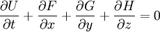
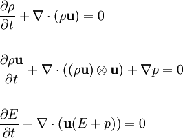
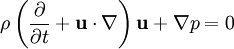
In fluid dynamics, the Euler equations govern the compressible, Inviscid flow. They correspond to the Navier-Stokes equations with zero viscosity and heat conduction terms, although they are usually written in the form shown here because this emphasises the fact that they directly represent conservation of mass, momentum, and energy. The equations are named after Leonhard Euler. This page assumes that classical mechanics applies; see relativistic Euler equations for a discussion of compressible fluid flow when velocities approach the speed of light. Additional recommended knowledgeAlthough the Euler equations formally reduce to potential flow in the limit of vanishing Mach number, this is not helpful in practice, essentially because the approximation of incompressibility is almost invariably very close. In differential form, the equations are: where E = ρe + ρ(u2 + v2 + w2) / 2 is the total energy per unit volume (e is the internal energy per unit mass for the fluid), u, v and w are the velocity components, p is the pressure, u the fluid velocity and ρ the fluid density. The second equation includes the divergence of a dyadic tensor, and may be clearer in subscript notation: Note that the above equations are expressed in conservation form, as this format emphasises their physical origins (and is by far the most convenient form for computational fluid dynamics simulations). The momentum component of the Euler equations is usually expressed as follows: but this form obscures the direct connection between the Euler equations and Newton's second law of motion (in particular, it is not intuitively clear why this equation is correct and where This form makes it clear that F,G,H are fluxes. The equations above thus represent conservation of mass, three components of momentum, and energy. There are thus five equations and six unknowns. Closing the system requires an equation of state; the most commonly used is the ideal gas law (i.e. p = ρ(γ − 1)e, where ρ is the density, γ the adiabatic index, and e the internal energy). Note the odd form for the energy equation; see Rankine-Hugoniot equation. The extra terms involving p may be interpreted as the mechanical work done on a fluid element by nearby fluid elements moving around. These terms sum to zero in an incompressible fluid. The better known Bernoulli's equation can be derived by integrating Euler's equation along a streamline under the assumption of constant density and a sufficiently stiff equation of state. Shock WavesThe Euler equations are nonlinear hyperbolic equations and their general solutions are waves. Much like the familiar oceanic waves, waves described by the Euler Equations 'break' and so-called shock waves are formed; this is a nonlinear effect and represents the solution becoming multi-valued. Physically this represents a breakdown of the assumptions that led to the formulation of the differential equations, and to extract further information from the equations we must go back to the more fundamental integral form. Then, weak solutions are formulated by working in 'jumps' (discontinuities) into the flow quantities - density, velocity, pressure, entropy - using the Rankine-Hugoniot shock conditions. Physical quantities are rarely discontinuous; in real flows, these discontinuities are smoothed out by viscosity. (See Navier-Stokes equations) Shock propagation is studied - among many other fields - in aerodynamics and rocket propulsion, where sufficiently fast flows occur. The Equations in One Space DimensionFor certain problems, especially when used to analyze compressible flow in a duct or in case the flow is cylindrically or spherically symmetric, the one-dimensional Euler equations are a useful first approximation. Generally, the Euler equations are solved by Riemann's method of characteristics. This involves finding curves in plane of independent variables (i.e., x,t) along which PDEs degenerate into ODEs. Numerical solutions of the Euler equations rely heavily on the method of characteristics. ReferencesThompson, Philip A. (1972). Compressible Fluid Flow. New York: McGraw-Hill. ISBN 0070644055. |
| This article is licensed under the GNU Free Documentation License. It uses material from the Wikipedia article "Euler_equations". A list of authors is available in Wikipedia. |


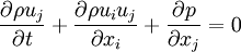
 is incorrect).
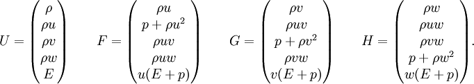
In conservation vector form, Euler equations become
is incorrect).
In conservation vector form, Euler equations become