To use all functions of this page, please activate cookies in your browser.
My watch list
my.chemeurope.com
my.chemeurope.com
With an accout for my.chemeurope.com you can always see everything at a glance – and you can configure your own website and individual newsletter.
- My watch list
- My saved searches
- My saved topics
- My newsletter
Fluctuation dissipation theoremIn statistical physics, the fluctuation dissipation theorem is a powerful tool for predicting the non-equilibrium behavior of a system — such as the irreversible dissipation of energy into heat — from its reversible fluctuations in thermal equilibrium. The fluctuation dissipation theorem applies both to classical and quantum mechanical systems. Although formulated originally by Nyquist in 1928[1], the fluctuation-dissipation theorem was first proved by Herbert B. Callen and Theodore A. Welton in 1951.[2] The fluctuation dissipation theorem relies on the assumption that the response of a system in thermodynamic equilibrium to a small applied force is the same as its response to a spontaneous fluctuation. Therefore, there is a direct relation between the fluctuation properties of the thermodynamic system and its linear response properties. Often the linear response takes the form of one or more exponential decays. Additional recommended knowledge
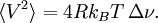
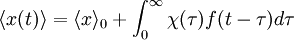
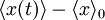
Example: Brownian motionFor example, Einstein in his 1905 paper on Brownian motion noted that the same random forces which cause the erratic motion of a particle in Brownian motion would also cause drag if the particle were pulled through the fluid. In other words, the fluctuation of the particle at rest has the same origin as the dissipative frictional force one must do work against, if one tries to perturb the system in a particular direction. From this observation he was able to use statistical mechanics to derive a previously unexpected connection, the Einstein-Smoluchowski relation: linking D, the diffusion constant, and μ, the mobility of the particles. (μ is the ratio of the particle's terminal drift velocity to an applied force, μ = vd / F). kB ≈ 1.38065 × 10⁻²³ m² kg s−2 K−1 is Boltzmann's constant, and T is the absolute temperature. Example: Thermal noise in a resistorIn 1928, John B. Johnson discovered and Harry Nyquist explained Johnson–Nyquist noise. With no applied current, the mean-square voltage depends on the resistance R, kBT, and the bandwidth Δν over which the voltage is measured: General applicabilityThe examples above turn out to be just two examples of a very general result in statistical thermodynamics, the fluctuation dissipation theorem, which can be used to give an explicit relationship between molecular dynamics at thermal equilibrium, and the macroscopic response that is observed in a dynamic measurement. It thus allows molecular scale models (microscopic models) to be used quantitatively to predict material properties in the context of linear response theory. The essence of fluctuation-dissipation theorem is that it relates equilibrium fluctuations to out-of-equilibrium quantities, like noise power is related to resistance. The theorem is based on fields that are weak relative to the potential of molecular interaction so that rates of relaxation are not affected by the applied field. "Out-of-equilibrium" in the above sentence should be understood as close to equilibrium or stationary states. General form of the fluctuation dissipation theoremThe fluctuation-dissipation theorem can be formulated in many ways; one particularly useful form is the following: Let x be an observable of a dynamical system with Hamiltonian H0(x) subject to thermal fluctuations. The observable x will fluctuate around its mean value < x > 0 with fluctuations characterized by a power spectrum Sx(ω). Suppose that we can switch on a (scalar) field f which alters the Hamiltionian to H(x) = H0(x) + xf. The response of the observable x to a field f(t) changing with time is characterized (to first order) by the susceptibility or linear response function χ(t) of the system
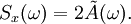
Now the fluctuation dissipation theorem relates the power spectrum to the imaginary part of the Fourier transform
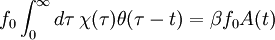
The left-hand side describes fluctuations in x, the right-hand side is closely related to the energy dissipated by the system when pumped by an oscillatory field f(t) = f0sin(ω). This theorem can be generalized in a straight-forward way to the case of space-dependent fields, to the case of several variables or to a quantum-mechanics setting. Violations of FDT in glassy systemsWhile the FDT provides a general relation between the response of equilibrium systems to small external perturbations and their spontaneous fluctuations, no general relation is known for systems out of equilibrium. In the mid 1990s, in the study of non-equilibrium dynamics of spin glass models it was discovered a generalization of FDT valid for asymptotic non-stationary states, where the temperature appearing in the equilibrium relation is substituted by an effective temperature with a non-trivial dependence on the time scales. This relation is proposed to hold in glassy systems beyond the models for which it was initially found. Derivation IWe derive the fluctuation dissipation theorem in the form given above, using the same notation. Consider the following test case: The field f has been on for infinite time and is switched off at t=0
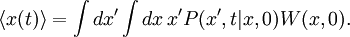
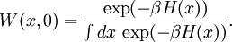
We can express the expectation value of x by the probablity distribution W(x,0) and the transition probability P(x',t | x,0) The probability distribution function W(x,0) is an equilibrium distribution and hence given by the Boltzmann distribution for the Hamiltionian H(x) = H0(x) + xf0 For a weak field here W0(x) is the equilibrium distribution in the absence of a field.
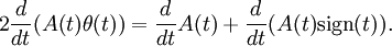
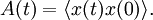
Plugging this approximation in the formula for where A(t) is the auto-correlation function of x in the absence of a field. Note that in the absence of a field the system is invariant under time-shifts.
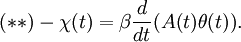
We can rewrite Consequently, For stationary processes, the Wiener-Khintchine theorem states, that the power spectrum equals twice the Fourier transform of the auto-correlation function The last step is to Fourier transform equation (**) and to take the
imaginary part. For this it is useful to recall that the Fourier transform
of a real symmetric function is real, while the Fourier transform of a real
antisymmetric function is purely imaginary.
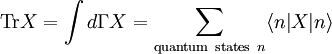
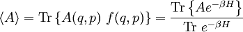
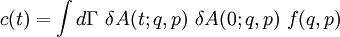
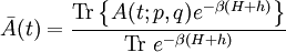
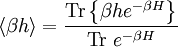
We can split Now the fluctuation dissipation theorem follows. Derivation IIThe following general derivation of the fluctuation-dissipation theorem uses averaging in phase space. The derivation applies equally well to classical as well as quantum mechanical systems, although the former uses a continuous integral over phase space, whereas the latter uses a sum over quantum states. To represent both, we introduce the trace notation, which applies both to classical and quantum systems where dΓ represents an infinitesimal volume in phase space. Thus, if a system is described by a probability distribution f(q, p) in phase space, the average value of an arbitrary function A of the system's state is given by where angular brackets are used to denote the averaging over the ensemble. In particular, if the probability distribution is given by the equilibrium Boltzmann distribution, the ensemble average equals where β = 1/kBT, kB is the Boltzmann constant and T is the temperature in Kelvin. Having defined our notation and basic variables, we now derive the fluctuation-dissipation theorem. Consider a system that has reached equilibrium under the Hamiltonian H + h, where h is much smaller than the thermal energy kBT. Being in thermal equilibrium, the probability of any state is proportional to its Boltzmann factor e−β(H + h). At time t = 0, let the perturbation h be turned off; given ergodicity, the system will gradually relax to a new equilibrium, which has Boltzmann factors e−βH. The fluctuation-dissipation theorem addresses the question of how quickly the system reaches its new equilibrium. Let the correlation function c(t) be defined which may be written as where δA(t; q, p) is the deviation from its mean at a time t, given that the system began at time t = 0 at position (q, p) in phase space. In other words, the integration is over all initial positions of the system in phase space. The mean value of A as it evolves towards its new equilibrium is given by Since h is much smaller than the thermal energy kBT, we may expand the numerator We may likewise expand the denominator where we have used which is much less than one, by our assumption that h is much smaller than the thermal energy 1/β = kBT. Combining the numerator and denominator, dropping quadratic and high-order terms in <βh>, and using the indifference of equilibrium to time, we obtain Let the perturbation h = −gA be proportional to the variable A with a constant −g. Then this formula becomes Note that the system's relaxation is independent of A and linear in g. These results imply that perturbations will relax independently of one another; if two perturbations, g1 and g2 are applied, the net relaxation will be the sum of the individual relaxations to g1 and g2 taken separately. Such continuous linear systems have been well-studied, and many methods developed for their solution, such as Fourier transforms and Laplace transforms. See also
References
Further resources
Categories: Statistical mechanics | Non-equilibrium thermodynamics |
|
| This article is licensed under the GNU Free Documentation License. It uses material from the Wikipedia article "Fluctuation_dissipation_theorem". A list of authors is available in Wikipedia. |


 .
.
 of the susceptibility
 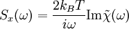 .
.
 , we can expand the right-hand side

 yields

 using the susceptibility
of the system and hence find with the above equation (*)
using the susceptibility
of the system and hence find with the above equation (*)
 into a symmetric and an
anti-symmetric part
into a symmetric and an
anti-symmetric part