To use all functions of this page, please activate cookies in your browser.
My watch list
my.chemeurope.com
my.chemeurope.com
With an accout for my.chemeurope.com you can always see everything at a glance – and you can configure your own website and individual newsletter.
- My watch list
- My saved searches
- My saved topics
- My newsletter
Grand canonical ensemble
In statistical mechanics, the grand canonical ensemble is a statistical ensemble (a large collection of identically prepared systems), where each system is in equilibrium with an external reservoir with respect to both particle and energy exchange. Therefore both the energy and the number of particles is allowed to fluctuate for each individual system in the ensemble. It is an extension of the canonical ensemble, where systems are only allowed to exchange energy (but not particles). And the chemical potential (or fugacity) is introduced to control the fluctuation of the number of particles. (Just like temperature is introduced into the canonical ensemble to control the fluctuation of energy.) It is convenient to use the grand canonical ensemble when the number of particles of the system cannot be easily fixed. Especially in quantum systems, e.g., a collection of bosons or fermions, the number of particles is an intrinsic property (rather than an external parameter) of each quantum state. And fixing the number of particles will cause certain mathematical inconvenience.
Additional recommended knowledge
The partition functionClassically, the partition function of the grand canonical ensemble is given as a weighted sum of canonical parition functions with different number of particles, where Quantum mechanically, the situation is even simpler (conceptually). For a system of bosons or fermions, it is often mathematically easier to treat the number of particles of the system as an intrinsic property of each quantum (eigen-)state, The parameter
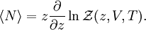
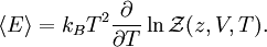
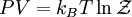
And the chemical potential is the Gibbs free energy per particle. (We haved used fugacity instead of chemical potential in defining the partition function. This is because fugacity is an independent parameter of partition function to control the number of particles, as temperature to control the energy. On the other hand, the chemical potential itself contains temperature dependence, which may lead to some confusion. ) Thermodynamic quantitiesThe average number of particles of the ensemble is obtained as And the average internal energy is
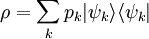
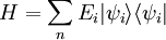
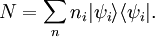
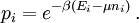
Statistics of bosons and fermionsFor a quantum mechanical system, the eigenvalues (energies) and the corresponding eigenvectors (eigenstates) of the Hamiltonian (the energy function) completely describe the system. For a macroscopic system, the number of eigenstates (microscopic states) is enormous. Statistical mechanics provides a way to average all microscopic states to obtain meaningful macroscopic quantities. The task of summing over states (calculating the partition function) appears to be simpler if we do not fix the total number of particles of the system. Because, for a noninteracting system, the partition function of grand canonical ensemble can be converted to a product of the partition functions of individual modes. This conversion makes the evaluation much easier. (However this conversion can not be done in canonical ensemble, where the total number of particles is fixed. ) Each mode is a spatial configuration for an individual particle. There may be none or some particles in each mode. In quantum mechanics, all particles are either bosons or fermions. For fermions, no two particles can share a same mode. But there is no such constraint for bosons. Therefore the partition function (of grand canonical ensemble) for each mode can be written as The Quantum mechanical ensembleAn ensemble of quantum mechanical systems is described by a density matrix. In a suitable representation, a density matrix ρ takes the form where pk is the probability of a system chosen at random from the ensemble will be in the microstate So the trace of ρ, denoted by Tr(ρ), is 1. This is the quantum mechanical analogue of the fact that the accessible region of the classical phase space has total probability 1. It is also assumed that the ensemble in question is stationary, i.e. it does not change in time. Therefore, by Liouville's theorem, [ρ, H] = 0, i.e. ρH = Hρ where H is the Hamiltonian of the system. Thus the density matrix describing ρ is diagonal in the energy representation. Suppose where Ei is the energy of the i-th energy eigenstate. If a system i-th energy eigenstate has ni number of particles, the corresponding observable, the number operator, is given by From classical considerations, we know that the state has (unnormalized) probability Thus the grand canonical ensemble is the mixed state The grand partition, the normalizing constant for Tr(ρ) to be 1, is |
||||||||
| This article is licensed under the GNU Free Documentation License. It uses material from the Wikipedia article "Grand_canonical_ensemble". A list of authors is available in Wikipedia. |


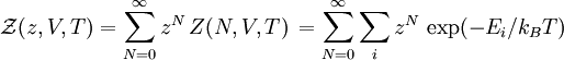
 denotes the partition function of the
  , of volume
  , and with the number of particles fixed at
  is the
  with energy
  . )
. )
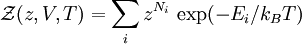
 is called
 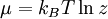 .
.
 and volume, divided by
 (some people use
  ) can be obtained as


 is the energy of the mode. For fermions,
  can be 0 or 1 (no particle or one particle in the mode). For bosons,
  . The upper (lower) sign is for fermions (bosons) in the last step. The total partition function is then a product of the ones for individual modes.


![{\mathcal Z} =\mathbf{Tr} [ e^{- \beta (H - \mu N)} ].](images/math/1/6/4/164ab7e0bf49179f7b14dd27adfd9bd9.png)


