To use all functions of this page, please activate cookies in your browser.
My watch list
my.chemeurope.com
my.chemeurope.com
With an accout for my.chemeurope.com you can always see everything at a glance – and you can configure your own website and individual newsletter.
- My watch list
- My saved searches
- My saved topics
- My newsletter
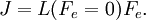
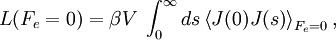
Green-Kubo relationsGreen-Kubo relations give exact mathematical expression for transport coefficients in terms of integrals of time correlation functions. Additional recommended knowledge
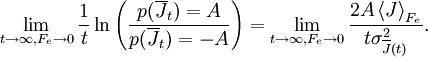
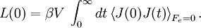
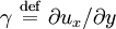
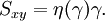
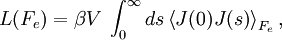
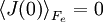
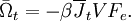
Thermal and mechanical transport processesThermodynamic systems may be prevented from relaxing to equilibrium because of the application of a mechanical field (e.g. electric or magnetic field), or because the boundaries of the system are in relative motion (shear) or maintained at different temperatures, etc. This generates two classes of nonequilibrium system: mechanical nonequilibrium systems and thermal nonequilibrium systems. The standard example of a mechanical transport process would be Ohm's law which states that at least for sufficiently small applied voltages, the current I is linearly proportional to the applied voltage V, As the applied voltage increases we expect to see deviations from linear behaviour. The coefficient of proportionality is the electrical conductivity which is the reciprocal of the electrical resistance. The standard example of a thermal transport process would be Newton's Law of viscosity which states that the shear stress Sxy is linearly proportional to the strain rate. The strain rate γ is the rate of change streaming velocity in the x-direction, with respect to the y-coordinate, As the strain rate increases we expect to see deviations from linear behaviour Another well known thermal transport process is Fourier's Law of Heat conduction which states that the heat flux between two bodies maintained at different temperatures is proportional to the temperature gradient (the temperature difference divided by the spatial separation). Linear constitutive relationsSo regardless of whether transport processes are stimulated thermally or mechanically, in the small field limit it is expected that a flux will be linearly proportional to an applied field. In such a case the flux and the force are said to be conjugate to each other. The relation between a thermodynamic force and its conjugate thermodynamic flux is called a linear constitutive relation, L(0) is called a linear transport coefficient. Green-Kubo relationsIn the 1950s M S Green and R Kubo proved an exact expression for linear transport coefficients which is valid for systems of arbitrary temperature, T, and density. They proved that linear transport coefficients are exactly related to the time dependence of equilibrium fluctuations in the conjugate flux, where β = 1 / (kT) with the Boltzmann constant k and V is the system volume. The integral is over the equilibrium flux autocorrelation function. At zero time the autocorrelation function is positive since it is the mean square value of the flux at equilibrium. [Note at equilibrium the mean value of the flux is zero by definition.] At long times the flux at time t, J(t), is uncorrelated with its value a long time earlier J(0) and the autocorrelation function decays to zero. This remarkable relation is frequently used in molecular dynamics computer simulation to compute linear transport coefficients—see Evans and Morriss "Statistical Mechanics of Nonequilibrium Liquids", Academic Press 1990, now available online. Nonlinear response and transient time correlation functionsIn 1985 Denis Evans and Morriss derived two exact fluctuation expressions for nonlinear transport coefficients—see Evans and Morriss Mol. Phys, 54, 629(1985). They proved that in a thermostatted system that is at equilibrium at t = 0, the nonlinear transport coefficient can be calculated from the so-called transient time correlation function expression: where the equilibrium (Fe = 0) flux autocorrelation function is replaced by a thermostatted field dependent transient autocorrelation function. At time zero Another exact fluctuation expression derived by Evans and Morriss is the so-called Kawasaki expression for the nonlinear response: The ensemble average of the right hand side of the Kawasaki expression is to be evaluated under the application of both the thermostat and the external field. At first sight the transient time correlation function (TTCF) and Kawasaki expression might appear to be of limited use—because of their innate complexity. However, the TTCF is quite useful in computer simulations for calculating transport coefficients. Both expressions can be used to derive new and useful fluctuation expressions quantities like specific heats, in nonequilibrium steady states. Thus they can be used as a kind of partition function for nonequilibrium steady states. Derivation of Green-Kubo relations from the fluctuation theorem and the central limit theoremFor a thermostatted steady state, time integrals of the dissipation function are related to the dissipative flux, J, by the equation We note in passing that the long time average of the dissipation function is a product of the thermodynamic force and the average conjugate thermodynamic flux. It is therefore equal to the spontaneous entropy production in the system. The spontaneous entropy production plays a key role in linear irreversible thermodynamics - see de Groot and Mazur "Non-equilibrium thermodynamics" Dover. The fluctuation theorem (FT) is valid for arbitrary averaging times, t. Let's apply the FT in the long time limit while simultaneously reducing the field so that the product Because of the particular way we take the double limit, the negative of the mean value of the flux remains a fixed number of standard deviations away from the mean as the averaging time increases (narrowing the distribution) and the field decreases. This means that as the averaging time gets longer the distribution near the mean flux and its negative, is accurately described by the central limit theorem. This means that the distribution is Gaussian near the mean and its negative so that Combining these two relations yields (after some tedious algebra!) the exact Green-Kubo relation for the linear zero field transport coefficient, namely, Details of the proof of Green-Kubo relations from the FT are here. SummaryThis shows the fundamental importance of the fluctuation theorem in nonequilibrium statistical mechanics. The FT (together with the Axiom of Causality) gives a generalisation of the Second Law of Thermodynamics. It is then easy to prove the second law inequality and the Kawasaki identity. When combined with the central limit theorem, the FT also implies the famous Green-Kubo relations for linear transport coefficients, close to equilibrium. The FT is however, more general than the Green-Kubo Relations because unlike them, the FT applies to fluctuations far from equilibrium. In spite of this fact, we have not yet been able to derive the equations for nonlinear response theory from the FT. The FT does not imply or require that the distribution of time-averaged dissipation is Gaussian. There are many examples known when the distribution is non-Gaussian and yet the FT (of course) still correctly describes the probability ratios. Categories: Thermodynamics | Statistical mechanics | Non-equilibrium thermodynamics |
|
| This article is licensed under the GNU Free Documentation License. It uses material from the Wikipedia article "Green-Kubo_relations". A list of authors is available in Wikipedia. |


 . Newton's Law of viscosity states

 but at later times since the field is applied
 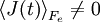 .
.
![\left\langle {J(t;F_e )} \right\rangle = \left\langle {J(0)\exp [ - \beta V\int_0^t {J( - s)F_e \;ds]} } \right\rangle _{F_e }. \,](images/math/8/5/e/85e25815d6fb33852561bcc50c70b55a.png)
 is held constant,