To use all functions of this page, please activate cookies in your browser.
My watch list
my.chemeurope.com
my.chemeurope.com
With an accout for my.chemeurope.com you can always see everything at a glance – and you can configure your own website and individual newsletter.
- My watch list
- My saved searches
- My saved topics
- My newsletter
Ising modelThe Ising model, named after the physicist Ernst Ising, is a mathematical model in statistical mechanics. It has since been used to model diverse phenomena in which bits of information, interacting in pairs, produce collective effects. Additional recommended knowledge
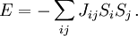
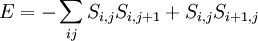
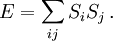
DefinitionThe Ising model is defined on a discrete collection of variables called spins, which can take on the value 1 or −1. The spins Si interact in pairs, with an energy which has one value when the two spins are the same, and a second value when the two spins are different. Energy functionThe energy of the Ising model is defined to be: Notice that the product of spins is either +1 if the two spins are the same, or aligned, and −1 if they are different, antialigned. J is half the difference in energy between the two possibilities. For each pair, if
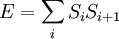
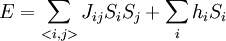
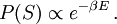
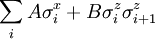
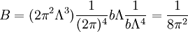
A ferromagnetic interaction tends to align spins, and an antiferromagnetic tends to antialign them. The spins can be thought of as living on a graph, where each node has exactly one spin, and each edge connects two spins with a nonzero value of J. If all the Js are equal, it is convenient to measure energy in units of J. Then a model is completely specified by the graph and the sign of J. Simple examplesThe antiferromagnetic one-dimensional Ising model has the energy function: where i runs over all the integers. This links each pair of nearest neighbors. The ferromagnetic two-dimensional Ising model on a square lattice is a collection of spins Si,j on each node (i,j) of a two dimensional square lattice and the Energy is: Notice that the sum links every site to its right-neighbor and its down-neighbor. In this way, every edge is only counted once. The mean field Ising model is the Ising model on a complete graph, where all the nodes are connected to all the other nodes: Magnetic fieldThe energy of the Ising model may be modified to bias the entire system. Normally, an Ising model is completely symmetric under interchange of + and −. A magnetic field hi may be added to the energy, and it breaks the symmetry, The full energy function is: where the brackets indicate that i and j index neighboring positions on the graph. StatisticsThe model is a statistical model, so the Energy is really the logarithm of the probability. The probability of each configuration of spins is the Boltzmann distribution with inverse temperature β. To actually generate configurations using this probability distribution is conceptually easiest using the Metropolis Algorithm:
The change in energy ΔE only depends on the value of the spin and its nearest graph neighbors. So if the graph is not too connected, the algorithm is fast. This process will eventually produce a pick from the distribution. QuestionsThe interesting statistical questions to ask are all in the limit of large numbers of spins:
General discussion
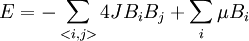
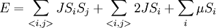
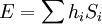
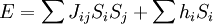
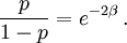
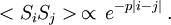
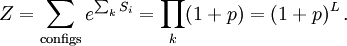
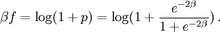
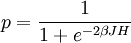
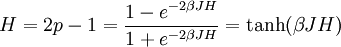
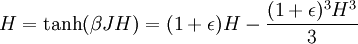
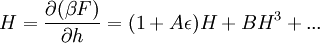
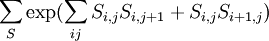
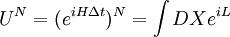
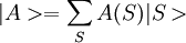
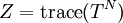
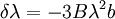
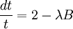
In his 1925 PhD thesis, Ising solved the model for the 1D case. In one dimension, the solution admits no phase transition. On the basis of this result, he incorrectly concluded that his model does not exhibit phase behaviour in any dimension. Most numerical solutions use the Metropolis-Hastings algorithm run inside a Monte Carlo loop. Depending on the complexity only adjacent vertices can be taken into account or for long-range models other vertices can be included. The Ising model undergoes a phase transition between an ordered and a disordered phase in 2 dimensions or more. In 2 dimensions, the Ising model has a strong/weak duality (between high temperatures and low ones) called the Kramers-Wannier duality. The fixed point of this duality is at the second-order phase transition temperature. While the Ising model is an extremely simplified description of ferromagnetism, its importance is underscored by the fact that other systems can be mapped exactly or approximately to the Ising system. The grand canonical ensemble formulation of the lattice gas model, for example, can be mapped exactly to the canonical ensemble formulation of the Ising model. The mapping allows one to exploit simulation and analytical results of the Ising model to answer questions about the related models. The Ising model on a two dimensional square lattice with no magnetic field was analytically solved in 1944 by Lars Onsager. Onsager showed that the correlation functions and free energy of the Ising model are locally determined by a noninteracting lattice fermion. The 3D Ising model does not have a representation in terms of free fields. In 2000, Sorin Istrail established that computing the free energy of the Ising model on an arbitrary sublattice of a three dimensional square lattice is computationally intractable.[1] While this means that it is impossible to efficiently compute all possible thermodynamic quantities with arbitrary external fields, it does not mean that the critical exponents or spin-spin correlations cannot be computed near criticality. In particular, Istrail's proof is valid in four or higher dimensions, where the model is also exactly solvable near criticality, since its correlation functions at long distances are those of a free scalar field. Physical systemsMagnetismThe original motivation for the model was the phenomenon of ferromagnetism. Iron is magnetic; once it is magnetized it stays magnetized for a long time compared to any atomic time. Since the 19th century, it was clear that magnetic fields are due to currents in matter, and Ampere postulated that permanent magnets are caused by permanent atomic currents. The motion of classical charged particles could not explain permanent currents though, as shown by Larmor. In order to have ferromagnetism, the atoms must have permanent magnetic moments which are not due to the motion of classical charges. Once the electron's spin was discovered, it was clear that the magnetism should be due to a large number of electrons spinning in the same direction. It was natural to ask how the electrons all know which direction to spin, because the electrons on one side of a magnet don't directly interact with the electrons on the other side. They can only influence their neighbors. The Ising model was designed to investigate whether a large fraction of the electrons could be made to spin in the same direction using only local forces. Lattice gasThe Ising model can be reinterpreted as a statistical model for the motion of atoms. Since the kinetic energy doesn't depend on the position only on the momentum, the statistics of the positions only depends on the potential energy, the thermodynamics of the gas only depends on the potential energy for each configuration of atoms. A coarse model is to make space-time a lattice and imagine that each position either contains an atom or it doesn't. The space of configuration is that of independent bits Bi, where each bit is either 0 or 1 depending on whether the position is occupied or not. An attractive interaction reduces the energy of two nearby atoms. If the attraction is only between nearest neighbors, the energy is reduced by − 4JBiBj for each occupied neighboring pair. The density of the atoms can be controlled by adding a chemical potential, which is a multiplicative probability cost for adding one more atom. A multiplicative factor in probability can be reinterpreted as an additive term in the logarithm – the energy. The extra energy of a configuration with N atoms is changed by μN. The probability cost of one more atom is a factor of exp( − βμ). So the energy of the lattice gas is: Rewriting the bits in terms of spins, Bi = (Si + 1) / 2. For lattices where every site has an equal number of neighbors, this is the Ising model with a magnetic field h = μ + KJ, where K is the number of neighbors. Neural activityThe activity of neurons in the brain can be modelled statistically. Each neuron at any time is either active + or inactive −. The active neurons are those that send an action potential down the axon in any given time window, and the inactive ones are those that do not. Because the neural activity at any one time is modelled by independent bits, Hopfield suggested that a dynamical Ising model would provide a first approximation to a neural network which is capable of learning.[2] A recent interpretation of Schneidman, Berry, Segev and Bialek [3] is that the Ising model is useful for any model of neural function, because a statistical model for neural activity should be chosen using the principle of maximum entropy. Given a collection of neurons, a statistical model which can reproduce the average firing rate for each neuron introduces a Lagrange multiplier for each neuron: But the activity of each neuron in this model is statistically independent. To allow for pair correlations, when one neuron tends to fire (or not to fire) along with another, introduce pair-wise lagrange multipliers: This energy function only introduces probability biases for a spin having a value and for a pair of spins having the same value. Higher order correlations are unconstrained by the multipliers. An activity pattern sampled from this distribution requires the largest number of bits to store in a computer, in the most efficient coding scheme imaginable, as compared with any other distribution with the same average activity and pairwise correlations. Mathematical developmentOne dimension – independent spin flipsThe energy of the one dimensional ferromagnetic Ising model is: Where i runs from 0 to L, where L is the length of the line. The energy of the lowest state is − L, when all the spins are the same. For any other configuration, the extra energy is equal to the number of sign changes as you scan the configuration from left to right. If we call the number of sign changes in a configuration k, the difference in energy from the lowest energy state is 2k. Since the energy is additive in the number of flips, the probability p of having a spin-flip at each position is independent. The ratio of the probability of finding a flip to the probability of not finding one is the Boltzmann factor: The problem is reduced to independent biased coin tosses. This essentially completes the mathematical description. From the description in terms of independent tosses, the statistics of the model for long lines can be understood. The line splits into domains. Each domain is of average length exp(2β). The length of a domain is distributed exponentially, since there is a constant probability at any step of encountering a flip. The domains never become infinite, so a long system is never magnetized. Each step reduces the correlation between a spin and its neighbor by an amount proportional to p, so the correlations fall off exponentially. The partition function is the volume of configurations, each configuration weighted by its Boltzmann weight. Since each configuration is described by a the sign-changes, the Partition function factorizes: The logarithm divided by L is the free energy density: which is analytic away from Infinite dimensions – mean fieldThe behavior of an Ising model on a fully connected graph may be completely understood by mean field theory. This type of description is appropriate to very high dimensional square lattices, because then each site has a very large number of neighbors. The idea is that if each spin is connected to a large number of spins, only the average number of + spins to − spins is important, since the fluctuations about this mean will be small. The mean field H is the average fraction of spins which are +. The energy cost of flipping a single spin in the mean field H is 2JNH. It is convenient to redefine J to absorb the factor N, so that the limit This energy cost gives the ratio of probability p that the spin is + to the probability 1-p that the spin is −. This ratio is the Boltzmann factor. so that The mean value of the spin is given by averaging 1 and −1 with the weights p and 1-p, so the mean value is 2p-1. But this average is the same for all spins, and is therefore equal to H. The solutions to this equation are the possible consistent mean fields. For βJ < 1 there is only the one solution at H=0. For bigger values of β there are three solutions, and the solution at H=0 is unstable. The instability means that increasing the mean field above zero a little bit produces a statistical fraction of spins which are + which is bigger than the value of the mean field. So a mean field which fluctuates above zero will produce an even greater mean field, and will eventually settle at the stable solution. This means that for temperatures below the critical value βJ = 1 the mean field Ising model undergoes a phase transition in the limit of large N. Above the critical temperature, fluctuations in H are damped because the mean field restores the fluctuation to zero field. Below the critical temperature, the mean field is driven to a new equilibrium value, which is either the positive H or negative H solution to the equation. For βJ = 1 + ε, just below the critical temperature, the value of H can be calculated from the Taylor expansion of the Hyperbolic tangent: dividing by H to discard the unstable solution at H=0, the stable solutions are: The spontaneous magnetization H grows near the critical point as the square root of the change in temperature. This is true whenever H can be calculated from the solution of an analytic equation which is symmetric between positive and negative values, which led Landau to suspect that all Ising type phase transitions in all dimensions should follow this law. The mean field exponent is universal because changes in the character of solutions of analytic equations are always described by catastrophies in the Taylor series, which is a polynomial equation. By symmetry, the equation for H must only have odd powers of H on the right hand side. Changing β should only smoothly change the coefficients. The transition happens when the coefficient of H on the right hand side is 1. Near the transition: Whatever A and B are, so long as neither of them is tuned to zero, the sponetaneous magnetization will grow as the square root of ε. This argument can only fail if the free energy βF is either non-analytic or non-generic at the exact β where the transition occurs. But the spontaneous magnetization in magnetic systems and the density in gasses near the critical point are measured very accuratedly. The density and the magnetization in three dimensions have the same power-law dependence on the temperature near the critical point, but the behavior from experiments is: The exponent is also universal, it is the same in the Ising model as in the experimental magnet and gas. but it is not equal to the mean field value. This was a great surprise. This is also true in two dimensions, where But there it was not a surprise, because it was predicted by Onsager. Two dimensions – Onsager's solutionThe partition function of the Ising model in two dimensions on a square lattice can be mapped to a two dimensional free fermion. This allows the specific heat to be calculated exactly. Transfer matrixStart with an analogy with quantum mechanics. The Ising model on a long periodic lattice has a partition function Think of the i direction as space, and the j direction as time. This is an independent sum over all the values that the spins can take at each time slice. This is a type of path integral, it is the sum over all spin histories. A path integral can be rewritten as a Hamiltonian evolution. The Hamiltonian steps through time by performing a unitary rotation between time t and time t + Δt: The product of the U matrices, one after the other, is the total time evolution operator, which is the path integral we started with. Where N is the number of time slices. The sum over all paths is given by a product of matrices, each matrix element is the transition probability from one slice to the next. Similarly, one can divide the sum over all partition function configurations into slices, where each slice is the one-dimensional configuration at time 1. This defines the transfer matrix: The configurations in each slice is a one dimensional collection of spins. At each time slice, T has matrix elements between two configurations of spins, one in the immediate future and one in the immediate past. These two configurations are C1 and C2, and they are all one dimensional spin configurations. We can think of the vector space that T acts on as all complex linear combinations of these. Using quantum mechanical notation: Where each basis vector | S > is a spin configuration of a one dimensional Ising model. Like the Hamiltonian, the transfer matrix acts on all linear combinations of states. The partition function is a matrix function of T, which is defined by the sum over all histories which come back to the original configuration after N steps: Since this is a matrix equation, it can be evaluated in any basis. So if we can diagonalize the matrix T, we can find Z. T in terms of Pauli matricesThe contribution to the partition function for each past/future pair of configurations on a slice is the sum of two terms. There is the number of spin flips in the past slice and there is the number of spin flips between the past and future slice. Define an operator on configurations which flips the spin at site i: In the usual Ising basis, acting on any linear combination of past configurations, it produces the same linear combination but with the spin at position i of each basis vector flipped. Define a second operator which multiplies the basis vector by +1 and −1 according to the spin at position i: T can be written in terms of these: Where A and B are constants which are to be determined so as to reproduce the partition function. The interpretation is that the statistical configuration at this slice contributes according to both the number of spin flips in the slice, and whether or not the spin at position i has flipped. Spin flip creation and annihilation operatorsJust as in the one dimensional case, we will shift attention from the spins to the spin-flips. The σz term in T counts the number of spin flips, which we can write in terms of spin-flip creation and annihilation operators: The first term flips a spin, so depending on the basis state it either:
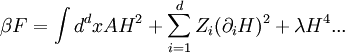
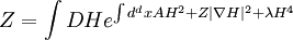
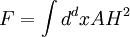
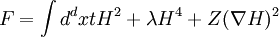
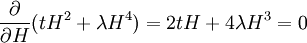
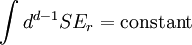
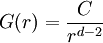
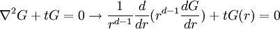
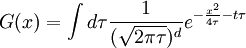
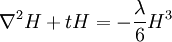
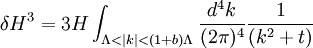
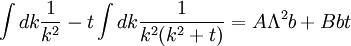
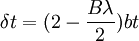
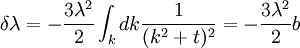
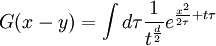
Writing this out in terms of creation and annihilation operators: Ignore the constant coefficients, and focus attention on the form. They are all quadratic. Since the coefficients are constant, this means that the T matrix can be diagonalized by Fourier transforms. Carrying out the diagonalization produces the Onsager free energy. Dimensions 5 and above – free fieldIn any dimension, the Ising model can be productively described by a locally varying mean field. The field is defined as the average spin value over a large region, but not so large so as to include the entire system. The field still has slow variations from point to point, as the averaging volume moves. These fluctuations in the field are described by a continuum field theory in the infinite system limit. Local fieldThe field H is defined as the long wavelength Fourier components of the spin variable, in the limit that the wavelengths are long. There are many ways to take the long wavelength average, depending on the details of how high wavelengths are cut off. The details are not too important, since the goal is to find the statistics of H and not the spins. Once the correlations in H are known, the long-distance correlations between the spins will be proportional to the long-distance correlations in H. For any value of the slowly varying field H, the free energy (log-probability) is a local analytic function of H and its gradients. The free energy F(H) is defined to be the sum over all Ising configurations which are consistent with the long wavelength field. Since H is a coarse description, there are many Ising configurations consistent with each value of H, so long as not too much exactness is required for the match. Since the allowed range of values of the spin in any region only depend on the values of H within one averaging volume from that region, the free energy contribution from each region only depends on the value of H there and in the neighboring regions. So F is a sum over all regions of a local contribution, which only depends on H and its derivatives. By symmetry in H, only even powers contribute. By reflection symmetry on a square lattice, only even powers of gradients contribute. Writing out the first few terms in the free energy assuming both k and H are small: On a square lattice, symmetries guarantee that the coefficients Zi of the derivative terms are all equal. But even for an anisotropic Ising model, where the Z's in different directions are different, the fluctuations in H are isotropic in a coordinate system where the different directions of space are rescaled. On any lattice, the derivative term Since βF is a function of a slowly spatially varying field. The probability of any field configuration is: The statistical average of any product of H's is equal to: The denominator in this expression is called the partition function, and the integral over all possible values of H is a statistical path integral. It integrates exp(βF) over all values of H, over all the long wavelength fourier components of the spins. F is a Euclidean Lagrangian for the field H, the only difference between this and the quantum field theory of a scalar field is that all the derivative terms enter with a positive sign, and there is no overall factor of i. Dimensional analysisThe form of F can be used to predict which terms are most important by dimensional analysis. Dimensional analysis is not completely straightforward, because the scaling of H needs to be determined. In the generic case, choosing the scaling law for H is easy. When k is small and H is small, the only term that contributes the first one, This term is the most significant, but it gives trivial behavior. This form of the free energy is ultralocal, meaning that it is a sum of an independent contribution from each point. This is like the spin-flips in the one-dimensional Ising model. Every value of H at any point fluctuates completely independently of the value at any other point. The scale of the field can be redefined to absorb the coefficient A, and then it is clear that A only determines the overall scale of fluctuations. The ultralocal model describes the long wavelength high temperature behavior of the Ising model, since in this limit the fluctuation averages are independent from point to point. To find the critical point, lower the temperature. As the temperature goes down, the fluctuations in H go up because the fluctuations are more correlated. This means that the average of a large number of spins does not become small as quickly as if they were uncorrelated, because they tend to be the same. This corresponds to decreasing A in the system of units where H does not absorb A. The phase transition can only happen when the subleading terms in F can contribute, but since the first term dominates at long distances, the coefficient A must be tuned to zero. This is the location of the critical point: Where t is a parameter which goes through zero at the transition. Since t is vanishing, fixing the scale of the field using this term makes the other terms blow up. Once t is small, the scale of the field can either be set to fix the coefficient of the H4 term or the MagnetizationTo find the magnetization, fix the scaling of H so that λ is one. Now the field H has dimension −d/4, so that H4ddx is dimensionless, and Z has dimension 2−d/2. In this scaling, the gradient term is only important at long distances for There is one subtle point. The field H is fluctuating statistically, and the fluctuations can shift the zero point of t. To see how, consider H4 split in the following way: The first term is a constant contribution to the free energy, and can be ignored. The second term is a finite shift in t. The third term is a quantity that scales to zero at long distances. This means that when analyzing the scaling of t by dimensional analysis, it is the shifted t that is important. This was historically very confusing, because the shift in t at any finite λ is finite, but near the transition t is very small. The fractional change in t is very large, and in units where t is fixed the shift looks infinite. The magnetization is at the minimum of the free energy, and this is an analytic equation. In terms of the shifted t, For t<0, the minima are at H proportional to the square root of t. So Landau's catastrophe argument is correct in dimensions larger than 5. The magnetization exponent in dimensions higher than 5 is equal to the mean field value. When t is negative, the fluctuations about the new minimum are described by a new positive quadratic coefficient. Since this term always dominates, at temperatures below the transition the flucuations again become ultralocal at long distances. FluctuationsTo find the behavior of fluctuations, rescale the field to fix the gradient term. Then the length scaling dimension of the field is 1−d/2. Now the field has constant quadratic spatial fluctuations at all temperatures. The scale dimension of the H2 term is 2, while the scale dimension of the H4 term is 4−d. For d<4, the H4 term has positive scale dimension. In dimensions higher than 4 it has negative scale dimensions. This is an essential difference. In dimensions higher than 4, fixing the scale of the gradient term means that the coefficient of the H4 term is less and less important at longer and longer wavelengths. The dimension at which nonquadratic contributions begin to contribute is known as the critical dimension. In the Ising model, the critical dimension is 4. In dimensions above 4, the critical fluctuations are described by a purely quadratic free energy at long wavelengths. This means that the correlation functions are all computable from as Gaussian averages: valid when x-y is large. The function G(x-y) is the analytic continuation to imaginary time of the Feynman propagator, since the free energy is the analytic continuation of the quantum field action for a free scalar field. For dimensions 5 and higher, all the other correlation functions at long distances are then determined by Wick's theorem. All the odd moments are zero, by +/- symmetry. The even moments are the sum over all partition into pairs of the product of G(x-y) for each pair. Where C is the proportionality constant. So knowing G is enough. It determines all the multipoint correlations of the field. The critical two point functionTo determine the form of G, consider that the fields in a path integral obey the classical equations of motion derived by varying the free energy: This is valid at noncoindent points only, since the correlations of H are singular when points collide. H obeys classical equations of motion for the same reason that quantum mechanical operators obey them – its fluctuations are defined by a path integral. At the critical point t=0, this is Laplace's equation, which can be solved by Gauss's method from electrostatics. Define an electric field analog by away from the origin: since G is spherically symmetric in d dimensions, E is the radial gradient of G. Integrating over a large d-1 dimensional sphere, This gives: and G can be found by integrating with respect to r. The constant C fixes the overall normalization of the field. G(r) away from the critical pointWhen t does not equal zero, so that H is fluctuating at a temperature slightly away from critical, the two point function decays at long distances. The equation it obeys is altered: For r small compared with To see how, it is convenient to represent the two point function as an integral, introduced by Schwinger in the quantum field theory context: This is G, since the fourier transform of this integral is easy. Each fixed τ contribution is a Gaussian in x, whose fourier transform is another Gaussian of reciprocal width in k. This is the inverse of the operator The interpretation of the integral representation over the proper time τ is that the two point function is the sum over all random walk paths that link position 0 to position x over time τ. The density of these paths at time τ at position x is Gaussian, but the random walkers disappear at a steady rate proportional to t so that the gaussian at time τ is diminished in height by a factor that decreases steadily exponentially. In the quantum field theory context, these are the paths of relativistically localized quanta in a formalism that follows the paths of individual particles. In the pure statistical context, these paths still appear by the mathematical correspondence with quantum fields, but their interpretation is less directly physical. The integral representation immediately shows that G(r) is positive, since it is represented as a weighted sum of positive Gaussians.
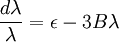
It also gives the rate of decay at large r, since the proper time for a random walk to reach position τ is r2
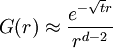
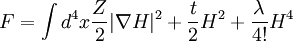
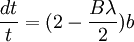
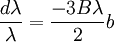
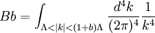
and in this time, the Gaussian height has decayed by A heuristic approximation for G(r) is: This is not an exact form, except in three dimensions, where interactions between paths become important. The exact forms in high dimensions are variants of Bessel functions. Symanzik polymer interpretationThe interpretation of the correlations as fixed size quanta travelling along random walks gives a way of understanding why the critical dimension of the H4 interaction is 4. The term H4 can be thought of as the square of the density of the random walkers at any point. In order for such a term to alter the finite order correlation functions, which only introduce a few new random walks into the fluctuating environment, the new paths must intersect. Otherwise, the square of the density is just proportional to the density and only shifts the H2 coefficient by a constant. But the intersection probability of random walks depends on the dimension, and random walks in dimension higher than 4 don't intersect. The fractal dimension of an ordinary random walk is 2. The number of balls of size ε required to cover the path increase as 1 / ε2. Two objects of fractal dimension 2 will intersect with reasonable probability only in a space of dimension 4 or less, the same condition as for a generic pair of planes. Kurt Symanzik argued that this implies that the critical Ising fluctuations in dimensions higher than 4 should be described by a free field. This argument eventually became a mathematical proof. 4-ε dimensions – renormalization groupThe Ising model in four dimensions is described by a fluctuating field, but now the fluctuations are interacting. In the polymer representation, intersections of random walks are marginally possible. In the quantum field continuation, the quanta interact. The negative logarithm of the probability of any field configuration H is the free energy function The numerical factors are there to simplify the equations of motion. The goal is to understand the statistical fluctuations. Like any other non-quadratic path integral, The correlation functions have a Feynman expansion as particles travelling along random walks, splitting and rejoining at vertices. The interaction strength is parametrized by the classically dimensionless quantity λ. Although dimensional analysis shows that both λ and Z dimensionless, this is misleading. The long wavelength statistical fluctuations are not exactly scale invariant, and only become scale invariant when the interaction strength vanishes. The reason is that there is a cutoff used to define H, and the cutoff defines the shortest wavelength. Fluctuations of H at wavelengths near the cutoff can affect the longer-wavelength fluctuations. If the system is scaled along with the cutoff, the parameters will scale by dimensional analysis, but then comparing parameters doesn't compare behavior because the rescaled system has more modes. If the system is rescaled in such a way that the short wavelength cutoff remains fixed, the long-wavelength fluctuations are modified. Wilson renormalizationA quick heuristic way of studying the scaling is to cut off the H wavenumbers at a point λ. Fourier modes of H with wavenumbers larger than λ are not allowed to fluctuate. A rescaling of length that make the whole system smaller increases all wavenumbers, and moves some fluctuations above the cutoff. To restore the old cutoff, perform a partial integration over all the wavenumbers which used to be forbidden, but are now fluctuating. In Feynman diagrams, integrating over a fluctuating mode at wavenumber k links up lines carrying momentum k in a correlation function in pairs, with a factor of the inverse propagator. Under rescaling, when the system is shrunk by a factor of (1+b), the t coefficient scales up by a factor (1+b)^2 by dimensional analysis. The change in t for infinitesimal b is 2bt. The other two coefficients are dimensionless and don't change at all. The lowest order effect of integrating out can be calculated from the equations of motion: This equation is an identity inside any correlation function away from other insertions. After integrating out the modes with Λ < k < (1 + b)Λ, it will be a slightly different identity. Since the form of the equation will be preserved, to find the change in coefficients it is sufficient to analyze the change in the H3 term. In a Feynman diagram expansion, the H3 term in a correlation function inside a correlation has three dangling lines. Joining two of them at large wavenumber k gives a change H3 with one dangling line, so proportional to H: The factor of 3 comes from the fact that the loop can be closed in three different ways. The integral should be split into two parts: the first part is not proportional to t, and in the equation of motion it can be absorbed by a constant shift in t. It is caused by the fact that the H3 term has a linear part. part is independent of the value of t. Only the second term, which varies from t to t, contributes to the critical scaling. This new linear term adds to the first term on the left hand side, changing t by an amount proportional to t. The total change in t is the sum of the term from dimensional analysis and this second term from operator products: So t is rescaled, but its dimension is anomalous, it is changed by an amount proportional to the value of λ. But λ also changes. The change in lambda requires considering the lines splitting and then quickly rejoining. The lowest order process is one where one of the three lines from H3 splits into three, which quickly joins with one of the other lines from the same vertex. The correction to the vertex is The numerical factor is three times bigger because there is an extra factor of three in choosing which of the three new lines to contract. So These two equations together define the renormalization group equations in four dimensions: The coefficient B is determined by the formula And is proportional to the area of a three dimensional sphere of radius λ, times the width of the integration region bΛ divided by Λ4 In other dimensions, the constant B changes, but the same constant appears both in the t flow and in the coupling flow. The reason is that the derivative with respect to t of the closed loop with a single vertex is a closed loop with two vertices. This means that the only difference between the scaling of the coupling and the t is the combinatorial factors from joining and splitting. Wilson Fisher pointTo investigate three dimensions starting from the four dimensional theory should be possible, because the intersection probabilities of random walks depend continuously on the dimensionality of the space. In the language of Feynman graphs, the coupling doesn't change very much when the dimension is changed. The process of continuing away from dimension four is not completely well defined without a prescription for how to do it. The prescription is only well defined on diagrams. It replaces the Schwinger representation in dimension 4 with the Schwinger representation in dimension 4 − ε defined by: In dimension 4 − ε, the coupling λ has positive scale dimension ε, and this must be added to the flow. The coefficient B is dimension dependent, but it will cancel. The fixed point for λ is no longer zero, but at: where the scale dimensions of t is altered by an amount λB = ε / 3. The magnetization exponent is altered proportionately to: which is .333 in 3 dimensions (ε = 1) and .166 in 2 dimensions (ε = 2). This is not so far off from the measured exponent .308 and the Onsager two dimensional exponent .125. Low dimensions – block spinsIn three dimensions, the perturbative series from the field theory is an expansion in a coupling constant λ which is not particularly small. The effective size of the coupling at the fixed point is one over the branching factor of the particle paths, so the expansion parameter is about 1/3. In two dimensions, the perturbative expansion parameter is 2/3. But renormalization can also be productively applied to the spins directly, without passing to an average field. Historically, this approach is due to Leo Kadanoff and predated the perturbative ε expansion. The idea is to integrate out lattice spins iteratively, generating a flow in couplings. But now the couplings are lattice energy coefficients. The fact that a continuum description exists guarantees that this iteration will converge to a fixed point when the temperature is tuned to criticality. Migdal-Kadanoff renormalizationWrite the two dimensional Ising model with an infinite number of possible higher order interactions. To keep spin reflection symmetry, only even powers contribute: By translation invariance, Jij is only a function of i-j. By the accidental rotational symmetry, at large i and j its size only depends on the magnitude of the two dimensional vector i-j. The higher order coefficients are also similarly restricted. The renormalization iteration divides the lattice into two parts – even spins and odd spins. The odd spins live on the odd-checkerboard lattice positions, and the even ones on the even-checkerboard. When the spins are indexed by the position (i,j), the odd sites are those with i+j odd and the even sites those with i+j even, and even sites are only connected to odd sites. The two possible values of the odd spins will be integrated out, by summing over both possible values. This will produce a new free energy function for the remaining even spins, with new adjusted couplings. The even spins are again in a lattice, with axes tilted at 45 degrees to the old ones. Unrotating the system restores the old configuration, but with new parameters. These parameters describe the interaction between spins at distances Starting from the Ising model and repeating this iteration eventually changes all the couplings. When the temperature is higher than critical, the couplings will converge to zero, since the spins at large distances are uncorrelated. But when the temperature is critical, there will be nonzero coefficients linking spins at all orders. The flow can be approximated by only considering the first few terms. This truncated flow will produce better and better approximations to the critical exponents when more terms are included. The simplest approximation is to keep only the usual J term, and discard everything else. This will generate a flow in J, analogous to the flow in t at the fixed point of λ in the ε expansion. To find the change in J, consider the four neighbors of an odd site. These are the only spins which interact with it. The multiplicative contribution to the partition function from the sum over the two values of the spin at the odd site is: Where N + ,N − are the number of neighbors which are + and −. Ignoring the factor of 2, the free energy contribution from this odd site is: This includes nearest neighbor and next-nearest neighbor interactions, as expected, but also a four-spin interaction which is to be discarded. To truncate to nearest neighbor interactions, consider that the difference in energy between all spins the same and equal numbers + and - is: Where D is the dimension of the lattice, D is three. From nearest neighbor couplings, the difference in energy between all spins equal and staggered spins is 8J. The difference in energy between all spins equal and nonstaggered but net zero spin is 4J. Ignoring four-spin interactions, a reasonable truncation is the average of these two energies or 6J. Since each link will contribute to two odd spins, the right value to compare with the previous one is half that: For small J, this quickly flows to zero coupling. Large J's flow to large couplings. The magnetization exponent is determined from the slope of the equation at the fixed point. Variants of this method produce good numerical approximations for the critical exponents when many terms are included, in two and three dimensions. See also
References
Categories: Statistical mechanics | Lattice models |
|
| This article is licensed under the GNU Free Documentation License. It uses material from the Wikipedia article "Ising_model". A list of authors is available in Wikipedia. |


 . A sign of a
  is smooth. In terms of the new J, the energy cost for flipping a spin is
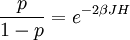


 is a positive definite quadratic form, and can be used to define the metric for space. So any translationally invariant Ising model is rotationally invariant at long distances, in coordinates that make
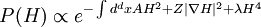

 term to 1.
 . Above four dimensions, at long wavelengths, the overall magnetization is only affected by the ultralocal terms.


 , the solution diverges exactly the same way as in the critical case, but the
long distance behavior is modified.
, the solution diverges exactly the same way as in the critical case, but the
long distance behavior is modified.
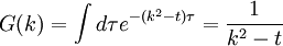
 in k space, acting on the unit function in k space, which is the fourier transform of a delta function source localized at the origin. So it satisfies the same equation as G with the same boundary conditions that determine the strength of the divergence at 0.
 . The decay factor appropriate for position r is therefore
  .
.


 larger.