To use all functions of this page, please activate cookies in your browser.
My watch list
my.chemeurope.com
my.chemeurope.com
With an accout for my.chemeurope.com you can always see everything at a glance – and you can configure your own website and individual newsletter.
- My watch list
- My saved searches
- My saved topics
- My newsletter
Lasing threshold
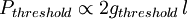
In a laser, the lasing threshold is the lowest excitation level at which the laser's output is dominated by stimulated emission rather than by spontaneous emission. Below the threshold, the laser's output power rises slowly with increasing excitation. Above threshold, the slope of power vs. excitation is orders of magnitude greater. The linewidth of the laser's emission also becomes orders of magnitude smaller above the threshold than it is below. Above the threshold, the laser is said to be lasing. Product highlightThe lasing threshold is reached when the optical gain of the laser medium is exactly balanced by the sum of all the losses experienced by light in one round trip of the laser's optical cavity. This can be expressed, assuming steady-state operation, as: Here R1 and R2 are the mirror (power) reflectivities, l is the length of the gain medium, The optical loss is nearly constant for any particular laser (α = α0), especially close to threshold. Under this assumption the threshold condition can be rearranged as: The first thing to note is that since R1R2 < 1, both terms on the right side are positive, hence both terms increase the required threshold gain parameter. It can be seen that minimising the gain parameter gthreshold requires low distributed losses and high reflectivity mirrors. This equation also suggests a benefit from using long gain media, i.e. high l. However this is not generally true. The dependence of the laser threshold on gain length requires a much more detailed analysis. The problem here is that longer gain lengths suffer from higher diffraction losses and so α is no longer constant but rather it increases. Anyway, generally, the gain medium length is not a free parameter in any experiment and so its effect on the threshold cannot be optimised. This simple analysis is predicated on the laser operating in a steady-state at laser threshold. However, this is not an assumption which can ever be fully satisfied. The problem is that the laser output power varies by orders of magnitude depending on which side of the threshold the laser is operating on. When very close to threshold, the smallest perturbation is able to cause huge swings in the output laser power. Nevertheless this formalism can be put to good use as follows. First let's make the assumption that one of the mirrors is perfectly reflecting; an assumption which is very good in many situations. Dielectric coatings routinely have reflectivities > 99.5% at the wavelengths of interest. Secondly let's call the second mirror, through which the laser output is transmitted, the output coupler. This element has a reflectivity denoted by ROC. Then we can write: It can be assumed that where we have used the relation L = 2α0l and K is a constant. This is the relationship we need. It allows the variable L to be determined. In order to use this expression, a series of slope efficiencies have to be obtained from a laser with each slope obtained with the laser using a different output coupler reflectivity. The power threshold is given by the intercept of each slope with the x-axis and must be found in each case. Next a graph of Pthreshold v − lnROC is plotted. The theory above suggests that this graph is a straight line. The line of best fit should be fitted to the data and the intercept of the line with the x-axis found. At this point the x value is equal to the round trip loss L = 2α0l. Now quantitative estimates of gthreshold can be made. One of the appealing features of this analysis is that all the measurements are made with the laser operating above the laser threshold. This allows for measurements with low random error to be made. However it does mean each estimate of Pthreshold requires extrapolation. The analysis presented here is in essence a Findlay-Clay analysis as published in 1966. A good empirical discussion of laser loss quantification is given in the book by W. Koechner. References
|
||
| This article is licensed under the GNU Free Documentation License. It uses material from the Wikipedia article "Lasing_threshold". A list of authors is available in Wikipedia. |


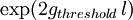 is the round-trip threshold (power) gain while
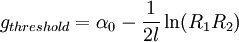

 where
where 


