To use all functions of this page, please activate cookies in your browser.
My watch list
my.chemeurope.com
my.chemeurope.com
With an accout for my.chemeurope.com you can always see everything at a glance – and you can configure your own website and individual newsletter.
- My watch list
- My saved searches
- My saved topics
- My newsletter
MUSCL schemeMUSCL stands for Monotone Upstream-centered Schemes for Conservation Laws, and the term was introduced in a seminal paper by Bram van Leer (van Leer, 1979). In this paper he constructed the first high-order, total variation diminishing (TVD) scheme where he obtained second order spatial accuracy. It is a finite volume method that provides high accuracy numerical solutions to partial differential equations which can involve solutions that exhibit shocks, discontinuities or large gradients. The idea is to replace the piecewise constant approximation of Godunov's scheme by reconstructed states, derived from cell-averaged states obtained from the previous time-step. For each cell, slope limited, reconstructed left and right states are obtained and used to calculate fluxes at the cell boundaries (edges). These fluxes can, in turn, be used as input to a Riemann solver, following which the solutions are averaged and used to advance the solution in time. Alternatively, the fluxes can be used in Riemann-free-solver schemes, such as the Kurganov and Tadmor scheme outlined below. Additional recommended knowledge
Linear reconstruction
We will consider the fundamentals of the MUSCL scheme by considering the following simple first-order, scalar, 1D system, which is assumed to have a wave propagating in the positive direction, Where The basic scheme of Godunov uses piecewise constant approximations for each cell, and results in a first-order upwind discretisation of the above problem with cell centres indexed as i. A semi-discrete scheme can be defined as follows,
This basic scheme is not able to handle shocks or sharp discontinuities as they tend to become smeared. An example of this effect is shown in the diagram opposite, which illustrates a 1D advective equation with a step wave propagating to the right. The simulation was carried out with a mesh of 200 cells and used a 4th order Runge-Kutta time integrator (RK-4). To provide higher resolution of discontinuities, Godunov's scheme can be extended to use piecewise linear approximations of each cell, which results in a central difference scheme that is second-order accurate in space. The piecewise linear approximations are obtained from
Thus, evaluating fluxes at the cell edges we get the following semi-discrete scheme
where
Whilst the above second-order scheme provides greater accuracy for smooth solutions, it is not a total variation diminishing (TVD) scheme and introduces spurious oscillations into the solution where discontinuities or shocks are present. An example of this effect is shown in the diagram opposite, which illustrates a 1D advective equation ut + ux = 0, with a step wave propagating to the right. This loss of accuracy is to be expected due to Godunov's theorem. The simulation was carried out with a mesh of 200 cells and used RK-4 for time integration.
MUSCL based numerical schemes extend the idea of using a linear piecewise approximation to each cell by using slope limited left and right extrapolated states. This results in the following high resolution, TVD discretisation scheme,
Which, alternatively, can be written in the more succinct form,
The numerical fluxes The symbols
and
The function The algorithm is straight forward to implement. Once a suitable scheme for Kurganov and Tadmor central schemeThe Nessyahu and Tadmor central scheme (Nessyahu and Tadmor, 1990) is a Riemann-solver-free, second-order, high-resolution scheme that uses MUSCL reconstruction. It is straight forward to implement and can be used on scalar and vector problems. The algorithm is based upon central differences with comparable performance to Riemann type solvers when used to obtain solutions for PDE’s describing systems that exhibit high-gradient phenomena. The Kurganov and Tadmor scheme can be implemented as a fully-discrete or semi-discrete scheme. Here we consider the semi-discrete scheme later proposed by Kurganov and Tadmor (2000) The calculation is shown below:
Where the local propagation speed,
where Beyond these CFL related speeds, no characteristic information is required. The above flux calculation is sometimes referred to as local Lax-Friedrichs flux or Rusanov flux (Lax, 1954; Rusanov, 1961; Toro, 1999; Kurganov and Tadmor, 2000; Leveque, 2002). An example of the effectiveness of using a high resolution scheme is shown in the diagram opposite, which illustrates the 1D advective equation The scheme can readily include diffusion terms, if they are present. For example, if the above 1D scalar problem is extended to include a diffusion term, we get
for which Kurganov and Tadmor propose the following central difference approximation,
Where,
Full details of the algorithm (full and semi-discrete versions) and its derivation can be found in the original paper (Kurganov and Tadmor, 1999), along with a number of 1D and 2D examples. Additional information is also available in an earlier related paper (Nessyahu and Tadmor, 1990). Note: Whilst this scheme was originally presented by Kurganov and Tadmor as a 2nd order scheme based upon linear extrapolation, a later paper (Kurganov and Levy, 2000) demonstrates that it can also form the basis of a third order scheme. A 1D advective example and a Euler equation example of their scheme, using parabolic reconstruction (3rd order), are shown in the parabolic reconstruction and Euler equation sections below. Piecewise parabolic reconstruction
It is possible to extend the idea of linear-extrapolation to higher order reconstruction, and an example is shown in the diagram opposite. However, for this case the left and right states are estimated by interpolation of a second-order, upwind biased, difference equation. This results in a parabolic reconstruction scheme that is third-order accurate in space. We follow the approach of Kermani (Kermani, et al, 2003), and present a third-order upwind biased scheme, where the symbols
and
Where
and the limiter function Parabolic reconstruction is straight forward to implement and can be used with the Kurganov and Tadmor scheme in lieu of the linear extrapolation shown above. This has the effect of raising the spatial solution of the KT scheme to 3rd order. It performs well when solving the Euler equations, see below. However, whilst this increase in spatial order has certain advantages over 2nd order schemes for smooth solutions, for shocks it is more disipative - compare diagram opposite with above solution obtained using the KT algorithm with linear extrapolation and Superbee limiter. This simulation was carried out on a mesh of 200 cells using the same KT algorithm but with parabolic reconstruction. Time integratration was by RK-4, and the alternative form of van Albada limiter, Euler equations exampleFor simplicity we consider the 1D case without heat transfer and without body force. Therefore, in conservation vector form, the general Euler equations reduce to
where
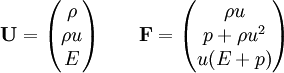
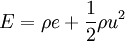
and where U is a vector of states and F is a vector of fluxes. The equations above represent conservation of mass, momentum, and energy. There are thus three equations and four unknowns, ρ (density) u (fluid velocity), p (pressure) and E (total energy). The total energy is given by,
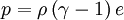
where In order to close the system an equation of state is required. One that suits our purpose is
where We can now proceed, as shown above in the simple 1D example, by obtaining the left and right extrapolated states for each state variable. Thus, for density we obtain
where
Having obtained the limited extrapolated states, we then proceed to construct the edge fluxes using these values. With the edge fluxes known, we can now construct the semi-discrete scheme, i.e.
The solution can now proceed by integration using standard numerical techniques. The above illustrates the basic idea of the MUSCL scheme. However, for a practical solution to the Euler equations, a suitable scheme has to be chosen which will also define the function
The diagram opposite shows a 2nd order solution to G A Sod's shock tube problem (Sod, 1978) using the above high resolution Kurganov and Tadmor Central Scheme (KT) with Linear Extrapolation and Ospre limiter. This illustrates clearly the effectiveness of the MUSCL approach to solving the Euler equations. The simulation was carried out on a mesh of 200 cells using Matlab code (Wesseling, 2001), adapted to use the KT algorithm and Ospre limiter. Time integration was performed by a 4th order SHK (equivalent performance to RK-4) integrator. The following initial conditions (SI units) were used:
The diagram opposite shows a 3rd order solution to G A Sod's shock tube problem (Sod, 1978) using the above high resolution Kurganov and Tadmor Central Scheme (KT) but with parabolic reconstruction and van Albada limiter. This again illustrates the effectiveness of the MUSCL approach to solving the Euler equations. The simulation was carried out on a mesh of 200 cells using Matlab code (Wesseling, 2001), adapted to use the KT algorithm with Parabolic Extrapolation and van Albada limiter. The alternative form of van Albada limiter,
More information on these and other methods can be found in the references below. References
Further reading
See also |
|
| This article is licensed under the GNU Free Documentation License. It uses material from the Wikipedia article "MUSCL_scheme". A list of authors is available in Wikipedia. |


 represents a state variable and
  represents a flux variable.
![\frac{d u_i}{d t} + \frac{1}{\Delta x_i} \left[ F \left( u_{i + 1} \right) - F \left( u_{i} \right) \right] =0](images/math/5/e/d/5ed0c6b5eb49d27deb7c73b828b19eb3.png) .
.
![u \left( x \right) = u_{i} + \frac{\left( x - x_{i} \right) }{ \left( x_{i+1} - x_{i} \right)} \left( u_{i+1} - u_{i} \right) , x \in \left[ x_{i}, x_{i+1} \right]](images/math/c/f/1/cf152c379a82b840e24feaad8914e4f8.png) .
.
![\frac{d u_i}{d t} + \frac{1}{\Delta x_i} \left[ F \left( u_{i + \frac{1}{2}} \right) - F \left( u_{i - \frac{1}{2}} \right) \right] =0](images/math/9/3/0/93033b6e2189976d69743b2de8a13c8c.png) ,
,
 and
and  are the piecewise approximate values of cell edge variables, i.e.
 ,
,
 .
.
![\frac{d u_i}{d t} + \frac{1}{\Delta x_i} \left[ F \left( u^*_{i + \frac{1}{2}} \right) - F \left( u^*_{i - \frac{1}{2}} \right) \right] =0](images/math/0/0/d/00d32d546944382b8204c02d896fc6cc.png) .
.
![\frac{d u_i}{d t} + \frac{1}{\Delta x_i} \left[ F^*_{i + \frac{1}{2}} - F^*_{i - \frac{1}{2}} \right] =0](images/math/1/2/d/12d24b803ddabacbe0b5bd80e4269022.png) .
.
 correspond to a nonlinear combination of first and second-order approximations to the continuous flux function.
 and
and  represent scheme dependent functions (of the limited extrapolated cell edge variables), i.e.
 ,
,
 ,
,
 ,
,
 .
.
 is a limiter function that limits the slope of the piecewise approximations to ensure the solution is TVD, thereby avoiding the spurious oscillations that would otherwise occur around discontinuities or shocks - see
  and is equal to unity when
  . Thus, the accuracy of a TVD discretization degrades to first order at local extrema, but tends to second order over smooth parts of the domain.
 has been chosen, such as the Kurganov and Tadmor scheme (see below), the solution can proceed using standard integration techniques such as Method of lines (MOL).
![F^*_{i-\frac{1}{2}} =\frac{1}{2} \left\{ \left[ F \left(u^R_{i - \frac{1}{2}} \right) + F \left(u^L_{i - \frac{1}{2}} \right) \right] - a_{i - \frac{1}{2} } \left[u^R_{i - \frac{1}{2}} - u^L_{i - \frac{1}{2}} \right] \right\}](images/math/f/0/b/f0b71c2c1e30ea53e55bc7a8e0b2a39a.png) .
.
![F^*_{i+\frac{1}{2}} =\frac{1}{2} \left\{ \left[ F \left(u^R_{i + \frac{1}{2}} \right) + F \left(u^L_{i + \frac{1}{2}} \right) \right] - a_{i + \frac{1}{2} } \left[u^R_{i + \frac{1}{2}} - u^L_{i + \frac{1}{2}} \right] \right\}](images/math/e/6/b/e6bf5a9fec344688c947682d1261ceef.png) .
.
 , is the maximum absolute value of the eigenvalue of the Jacobian of
  over cells
  given by
![a_{i \pm \frac{1}{2} } \left( t \right) = \max \left[ \rho \left( \frac{\partial F \left( u_{i} \left( t \right) \right)}{\partial u} \right) , \rho \left( \frac{\partial F \left( u_{i \pm 1} \left( t \right) \right)}{\partial u} \right) \right]](images/math/8/3/e/83e05100dfa7ad9d2cfbcbb329c962ba.png) ,
,
 represents the spectral radius of
 .
.
 , with a step wave propagating to the right. The simulation was carried out on a mesh of 200 cells, using the Kurganov and Tadmor central scheme with
 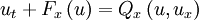 ,
,
![\frac{d u_i}{d t} = - \frac{1}{\Delta x_i} \left[ F^*_{i + \frac{1}{2}} - F^*_{i - \frac{1}{2}} \right] + \frac{1}{\Delta x_i} \left[ P_{i + \frac{1}{2}} - P_{i - \frac{1}{2}} \right]](images/math/d/8/c/d8c39503a00d9392c2417f72ff70a8c3.png) .
.
![P_{i + \frac{1}{2}} = \frac{1}{2} \left[ Q \left( u_{i} , \frac{u_{i+1} - u_i}{\Delta x_i} \right) + Q \left( u_{i+1} , \frac{u_{i+1} - u_i}{\Delta x_i} \right) \right]](images/math/1/5/d/15d43b55a055b44fb4d4f4d595411f29.png) ,
,
![P_{i - \frac{1}{2}} = \frac{1}{2} \left[ Q \left( u_{i-1} , \frac{u_{i} - u_{i-1}}{\Delta x_{i-1}} \right) + Q \left( u_{i} , \frac{u_{i} - u_{i-1}}{\Delta x_{i-1}} \right) \right]](images/math/9/9/8/9981b5fa775d9511a9867403143a3d32.png) .
.
 ,
,
![u^L_{i + \frac{1}{2}} = u_{i} + \frac{\phi \left( r_{i} \right)}{4} \left[ \left( 1 - \kappa \right) \delta u_{i - \frac{1}{2} } + \left( 1 + \kappa \right) \delta u_{i + \frac{1}{2} } \right]](images/math/e/f/b/efb95ca2abb1d20d0284912d4e951541.png) ,
,
![u^R_{i + \frac{1}{2}} = u_{i+1} - \frac{\phi \left( r_{i+1} \right)}{4} \left[ \left( 1 - \kappa \right) \delta u_{i + \frac{3}{2} } + \left( 1 + \kappa \right) \delta u_{i + \frac{1}{2} } \right]](images/math/5/5/4/5540c04f9e4596533cd51e293adf47e4.png) ,
,
![u^L_{i - \frac{1}{2}} = u_{i-1} + \frac{\phi \left( r_{i-1} \right)}{4} \left[ \left( 1 - \kappa \right) \delta u_{i - \frac{3}{2}} + \left( 1 + \kappa \right) \delta u_{i - \frac{1}{2} } \right]](images/math/0/2/5/025710074355be64cc13c427dd6ba712.png) ,
,
![u^R_{i - \frac{1}{2}} = u_{i} - \frac{\phi \left( r_{i} \right)}{4} \left[ \left( 1 - \kappa \right) \delta u_{i + \frac{1}{2} } + \left( 1 + \kappa \right) \delta u_{i - \frac{1}{2} } \right]](images/math/7/4/1/741ebee021c262de5aaf4741e8b70c24.png) .
.
 = 1/3 and,
 ,
,
 ,
,
 , is the same as above.
 , was used to avoid spurious oscillations.
 ,
,
 ,
,
 ,
,
 represents specific internal energy.
 ,
,
 is equal to the ratio of specific heats
 ![\left[ c_p/c_v \right]](images/math/4/e/4/4e405c6b8a4f0c34cbee2cdd8281149e.png) for the fluid.
for the fluid.
 ,
,
 ,
,
 .
.
![\frac{d \mathbf{U}_i}{d t} = - \frac{1}{\Delta x_i} \left[ \mathbf{F}^*_{i + \frac{1}{2} } - \mathbf{F}^*_{i - \frac{1}{2}} \right]](images/math/9/a/e/9ae5283a8a1a5161452e02e316a951ed.png) .
.
 .
.


