To use all functions of this page, please activate cookies in your browser.
My watch list
my.chemeurope.com
my.chemeurope.com
With an accout for my.chemeurope.com you can always see everything at a glance – and you can configure your own website and individual newsletter.
- My watch list
- My saved searches
- My saved topics
- My newsletter
Path integral formulation
The path integral formulation of quantum mechanics is a description of quantum theory which generalizes the action principle of classical mechanics. It replaces the classical notion of a single, unique history for a system with a sum, or functional integral, over an infinity of possible histories to compute a quantum amplitude. The path integral formulation was developed in 1948 by Richard Feynman. Some preliminaries were worked out earlier, in the course of his doctoral thesis work with John Archibald Wheeler. This formulation has proved crucial to the subsequent development of theoretical physics, since it provided the basis for the grand synthesis of the 1970s called the renormalization group which unified quantum field theory with statistical mechanics. If we realize that the Schrödinger equation is essentially a diffusion equation with an imaginary diffusion constant, then the path integral is a method for the enumeration of random walks. For this reason path integrals had also been used in the study of Brownian motion and diffusion before they were introduced in quantum mechanics.
Additional recommended knowledge
Formulating quantum mechanicsThe path integral method is an alternative formulation of quantum mechanics. The canonical approach, pioneered by Erwin Schrödinger, Werner Heisenberg and Paul Dirac paid great attention to wave-particle duality and the resulting uncertainty principle by replacing Poisson brackets of classical mechanics by commutators between operators in quantum mechanics. The Hilbert space of quantum states and the superposition law of quantum amplitudes follows. The path integral starts from the superposition law, and exploits wave-particle duality to build a generating function for quantum amplitudes. Abstract formulationFeynman proposed the following postulates:
In order to find the overall probability amplitude for a given process, then, one adds up, or integrates, the amplitude of postulate 3 over the space of all possible histories of the system in between the initial and final states, including histories that are absurd by classical standards. In calculating the amplitude for a single particle to go from one place to another in a given time, it would be correct to include histories in which the particle describes elaborate curlicues, histories in which the particle shoots off into outer space and flies back again, and so forth. The path integral assigns all of these histories amplitudes of equal magnitude but with varying phase, or argument of the complex number. The contributions that are wildly different from the classical history are suppressed only by the interference of similar, canceling histories (see below). The mathematical technique of path integrals does not imply that real particles must actually follow the paths so constructed. Mathematical expansions of functions by other functions are a general technique, and as such the functions used are not required to have any physical interpretation at all. They are usually constructed for mathematical convenience, with no necessary analogy to the physical model that they are modeling. Indeed, in the case of the Feynman path integral, the integration is over imaginary time, so the relevance of the paths to the particle's real physical path is open to debate. Feynman showed that his formulation of quantum mechanics is equivalent to the canonical approach to quantum mechanics. An amplitude computed according to Feynman's principles will also obey the Schrödinger equation for the Hamiltonian corresponding to the given action. Recovering the action principleFeynman was extending a classic paper by Paul Dirac on the quantum equivalent of the classical action principle. Dirac knew from earlier semiclassical work that the Maupertuis action, the action-angle variable action, is the classical analog of the phase of the wavefunction in an energy eigenstate. He noted that the transformation between the Maupertuis action and the usual Lagrange action replaces a description of a motion at fixed energy with description of a motion evolving between two fixed times. The phase interpretation of the Maupertuis action implied that the Lagrange action was also a phase, and that it was associated to an infinitesimal path starting and ending at two nearby positions at two nearby times. He noted that the full quantum transition amplitude between two points at two times can be heuristically thought of as a sum of this phase factor over all possible paths, where the phase over each infinitesimal segment is given by the Lagrange action. Dirac's work was only heuristic because he did not provide a precise prescription to calculate the sum, and he did not show that one could recover the Schrodinger equation or the canonical commutation relations from this rule. This was done by Feynman. Both noted that in the limit of action that is large compared to Planck's constant Classical action principles are puzzling because of their seemingly teleological quality: instead of predicting the future from initial conditions, they give a combination of initial conditions and final conditions to find the path inbetween, as if the system somehow knows where it's going to end up. The path integral explains why this works. The system doesn't have to know in advance where it's going; the path integral simply calculates the probability amplitude for any given process, and the path goes everywhere. After a long enough time, interference effects guarantee that only the contributions from the stationary points of the action give histories with appreciable probabilities. Concrete formulationFeynman's postulates are somewhat ambiguous in that they do not define what an "event" is or the exact proportionality constant in postulate 3. The proportionality problem can be solved by simply normalizing the path integral by dividing the amplitude by the square root of the total probability for something to happen (resulting in that the total probability given by all the normalized amplitudes will be 1, as we would expect). Generally speaking one can simply define the "events" in an operational sense for any given experiment. The equal magnitude of all amplitudes in the path integral tends to make it difficult to define it such that it converges and is mathematically tractable. For purposes of actual evaluation of quantities using path-integral methods, it is common to give the action an imaginary part in order to damp the wilder contributions to the integral, then take the limit of a real action at the end of the calculation. In quantum field theory this takes the form of Wick rotation. There is some difficulty in defining a measure over the space of paths. In particular, the measure is concentrated on "fractal-like" distributional paths. Time-slicing definitionFor a particle in a smooth potential, the path integral is approximated by Feynman as the small-step limit over zig-zag paths, which in one dimension is a product of ordinary integrals. For the motion of the particle from position x0 at time 0 to xn at time t, the time interval can be divided up into n little segments of fixed duration Δt. This process is called time slicing. An approximation for the path integral can be computed as proportional to where H is the entire history in which the particle zigzags from its initial to its final position linearly between all the values of In the limit of n going to infinity, this becomes a functional integral.
This limit does not, however, exist for the most important quantum-mechanical systems, the atoms, due to the
singularity of the Coulomb potential Canonical Commutation RelationsThe formulation of the path integral does not make it clear at first sight that the quantities x and p do not commute. In the path integral, these are just integration variables and they have no obvious ordering. Feynman discovered that the non-commutativity is still there [3] . To see this, consider the simplest path integral, the brownian walk. This is not yet quantum mechanics, so in the path-integral the action is not multiplied by i: The quantity x(t) is fluctuating, and the derivative is defined as the limit of a discrete difference. Note that the distance that a random walk moves is proportional to This shows that the random walk is not differentiable, since the ratio that defines the derivative diverges with probability one. The quantity In ordinary calculus, the two are only different by an amount which goes to zero as ε goes to zero. But in this case, the difference between the two is not zero: give a name to the value of the difference for any one random walk: and note that f(t) is a rapidly fluctuating statistical quantity whose average value is 1. The fluctuations of such a quantity can be described by a statistical Lagrangian Defining the time order to be the operator order: This is called the Ito lemma in stochastic calculus, and the (euclideanized) canonical commutation relations in physics. For a general statistical action, a similar argument shows that And in quantum mechanics, the extra i in the action converts this to the canonical commutation relation. Particle in curved spaceFor a particle in curved space the kinetic term depends on the position and the above time slicing cannot be applied, this being a manifestation of the notorious operator ordering problem in Schrödinger quantum mechanics. One may, however, solve this problem by transforming the time-sliced flat-space path integral to curved space using a multivalued coordinate transformation (nonholonomic mapping explained here). The path integral and the partition functionThe path integral is just the generalization of the integral above to all quantum mechanical problems—
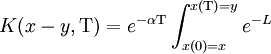
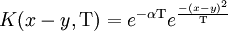
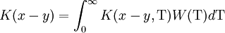
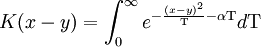
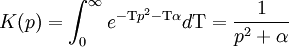
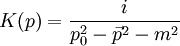
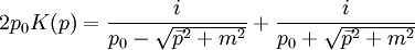
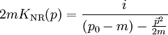
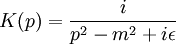
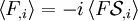
is the action of the classical problem in which one investigates the path starting at time t=0 and ending at time t = T, and Dx denotes integration over all paths. In the classical limit, The connection with statistical mechanics follows. Considering only paths which begin and end in the same configuration, perform the Wick rotation t→it, i.e., make time imaginary, and integrate over all possible beginning/ending configurations. The path integral now resembles the partition function of statistical mechanics defined in a canonical ensemble with temperature Clearly, such a deep analogy between quantum mechanics and statistical mechanics cannot be dependent on the formulation. In the canonical formulation, one sees that the unitary evolution operator of a state is given by where the state α is evolved from time t=0. If one makes a Wick rotation here, and finds the amplitude to go from any state, back to the same state in (imaginary) time iT is given by which is precisely the partition function of statistical mechanics for the same system at temperature quoted earlier. One aspect of this equivalence was also known to Schrödinger who remarked that the equation named after him looked like the diffusion equation after Wick rotation. Quantum field theoryThe path integral formulation was very important for the development of quantum field theory. Both the Schrodinger and Heisenberg approaches to quantum mechanics single out time, and are not in the spirit of relativity. For example, the Heisenberg approach requires that scalar field operators obey the commutation relation for x and y two simulataneous spatial positions, and this is not a relativistically invariant concept. The results of a calculation are covariant at the end of the day, but the symmetry is not apparent in intermediate stages. If naive field theory calculations did not produce infinite answers in the continuum limit, this would not have been such a big problem--- it would just have been a bad choice of coodinates. But the lack of symmetry means that the infinite quantities must be cut off, and the bad coordinates makes it nearly impossible to cut off the theory without spoiling the symmetry. This makes it difficult to extract the physical predictions, which require a careful limiting procedure. The problem of lost symmetry also appears in classical mechanics, where the Hamiltonian formulation also superficially singles out time. The Lagrangian formulation makes the relativistic invariance apparent. In the same way, the path integral is manifestly relativistic. It reproduces the Schrodinger equation as the evolution equation for the state at each time slice, and it also includes the Heisenberg equations of motion as a differential identity obeyed by averages of the integration variables at nearby times. It includes the canonical commutation relations in a natural way, and it extends them using the relativistic symmetry to operator product rules which are new relations difficult to extract from the old formalism. Further, different choices of canonical variables lead to very different seeming formulations of the same theory. The transformations between the variables can be very complicated, but the path integral makes them into reasonably straightforward changes of integration variables. For these reason, the Feynman path integral has made earlier formalisms largely obsolete. The price of a path integral representation is that the unitarity of a theory is no longer self evident, but it can be proven by changing variables to some canonical representation. The path integral itself also deals with larger mathematical spaces than is usual, which requires more careful mathematics not all of which has been fully worked out. The path integral historically was not immediately accepted, partly because it took many years to incorporate fermions properly. This required physicists to invent an entirly new mathematical object--- the grassman variable--- which also allowed changes of variables to be done naturally, as well as allowing constrained quantization. The integration variables in the path integral are subtly non-commuting. The value of the product of two field operators at what looks like the same point depends on how the two points are ordered in space and time. This makes some naive identities fail. The propagatorIn relativistic theories, there is both a particle and field representation for every theory. The field representation is a a sum over all field configurations, and the particle representation is a sum over different particle paths. The nonrelativistic formulation is traditionally given in terms of particle paths, not fields. There, the path integral in the usual variables, with fixed boundary conditions, gives the probability amplitude for a particle to go from point x to point y in time T. This is called the propagator. Superposing different values of the initial position x with an arbitrary initial state ψ0(x) constructs the final state. For a spatially homogenous system, where K(x,y) is a only a function of (x-y), the integral is a convolution, the final state is the initial state convolved with the propagator. For a free particle of mass m, the propagator can be evaluated either explicitly from the path integral or by noting that the Schrodinger equation is a diffusion equation in imaginary time and the solution must be a normalized Gaussian: Taking the Fourier transform in (x-y) produces another Gaussian: and in p-space the proportionality factor here is constant in time, as will be verified in a moment. The Fourier transform in time, extending K(p;T) to be zero for negative times, gives the Green's Function, or the frequency space propagator: Which is the reciprocal of the operator which annihilates the wavefunction in the Schrodinger equation, which wouldn't have come out right if the proportionality factor weren't constant in the p-space representation. The infinitesimal term in the denominator is a small positive number which guarantees that the inverse Fourier transform in E will be nonzero only for future times. For past times, the inverse Fourier transform contour closes toward values of E where there is no singularity. This guarantees that K propagates the particle into the future and is the reason for the subscript on G. The infinitesimal term can be interpreted as an infinitesimal rotation toward imaginary time. It is also possible to reexpress the nonrelativistic time evolution in terms of propagators which go toward the past, since the Schrodinger equation is time-reversible. The past propagator is the same as the future propagator except for the obvious difference that it vanishes in the future, and in the gaussian t is replaced by − t. In this case, the interpretation is that these are the quantities to convolve the final wavefunction so as to get the initial wavefunction. Given the nearly identical only change is the sign of E and \epsilon. The parameter E in the Green's function can either be the energy if the paths are going toward the future, or the negative of the energy if the paths are going toward the past. For a nonrelativistic theory, the time as measured along the path of a moving particle and the time as measured by an outside observer are the same. In relativity, this is no longer true. For a relativistic theory the propagator should be defined as the sum over all paths which travel between two points in a fixed proper time, as measured along the path. These paths describe the trajectory of a particle in space and in time. The integral above is not trivial to interpret, because of the square root. Fortunately, there is a heuristic trick. The sum is over the relativistic arclength of the path of an oscillating quantity, and like the nonrelativistic path integral should be interpreted as slightly rotated into imaginary time. The function K(x-y,\tau) can be evaluated when the sum is over paths in Euclidean space. This describes a sum over all paths of length Τ of the exponential of minus the length. This can be given a probability interpretation. The sum over all paths is a probability average over a path constructed step by step. The total number of steps is proportional to Τ, and each step is less likely the longer it is. By the central limit theorem, the result of many independent steps is a Gaussian of variance proportional to Τ. The usual definition of the relativistic propagator only asks for the amplitude is to travel from x to y, after summing over all the possible proper times it could take. Where W(Τ) is a weight factor, the relative importance of paths of different proper time. By the translation symmetry in proper time, this weight can only be an exponential factor, and can be absorbed into the constant α. This is the Schwinger representation. Taking a Fourier transform over the variable x − y can be done for each value of Τ separately, and because each separate Τ contribution is a Gaussian, gives whose fourier transform is another Gaussian with reciprocal width. So in p-space, the propagator can be reexpressed simply: Which is the Euclidian propagator for a scalar particle. Rotating p0 to be imaginary gives the usual relativistic propagator, up to a -i and an ambiguity which will be clarified below. This expression can be interpreted in the nonrelativistic limit, where it is convenient to split it by partial fractions: For states where one nonrelativistic particle is present, the initial wavefunction has a frequency distribution concentrated near p0 = m. When convolving with the propagator, which in p space just means multiplying by the propagator, the second term is supressed and the first term is enhanced. For frequencies near p0 = m, the dominant first term has the form: This is the expression for the Nonrelativistic Green's function of a free Schrodinger particle. The second term has a nonrelativistic limit also, but this limit is concentrated on frequencies which are negative. The second pole is dominated by contributions from paths where the proper time and the coordinate time are ticking in an opposite sense, which means that the second term is to be interpreted as the antiparticle. The nonrelativistic analysis shows that with this form the antiparticle still has positive energy. The proper way to express this mathematically is that, adding a small supression factor in proper time, the limit where Without these terms, the pole contribution could not be unambiguously evaluated when taking the inverse Fourier transform of p0. The terms can be recombined: Which when factored, produces opposite sign infinitesimal terms in each factor. This is the mathematically precise form of the relativistic particle propagator, free of any ambiguities. The ε term introduces a small imaginary part to the α = m2, which in the Minkowski version is a small exponential suppresion of long paths. So in the relativistic case, the Feynman path-integral representation of the propagator includes paths which go backwards in time, which describe antiparticles. The paths which contribute to the relativistic propagator go forward and backwards in time, and the interpretation of this is that the amplitude for a free particle to travel between two points includes amplitudes for the particle to fluctuate into an antiparticle, travel back in time, then forward again. Unlike the nonrelativistic case, it is impossible to produce a relativistic theory of local particle propagation without including antiparticles. All local differential operators have inverses which are nonzero outside the lightcone, meaning that it is impossible to keep a particle from travelling faster than light. Such a particle cannot be have a Greens function which is only nonzero in the future in a relativistically invariant theory. Functionals of fieldsHowever, the path integral formulation is also extremely important in direct application to quantum field theory, in which the "paths" or histories being considered are not the motions of a single particle, but the possible time evolutions of a field over all space. The action is referred to technically as a functional of the field: Much of the formal study of QFT is devoted to the properties of the resulting functional integral, and much effort (not yet entirely successful) has been made toward making these functional integrals mathematically precise. Such a functional integral is extremely similar to the partition function in statistical mechanics. Indeed, it is sometimes called a partition function, and the two are essentially mathematically identical except for the factor of i in the exponent in Feynman's postulate 3. Analytically continuing the integral to an imaginary time variable (called a Wick rotation) makes the functional integral even more like a statistical partition function, and also tames some of the mathematical difficulties of working with these integrals. Expectation valuesIn quantum field theory, if the action is given by the functional The symbol Schwinger-Dyson equationsSince this formulation of quantum mechanics is analogous to classical action principles, one might expect that identities concerning the action in classical mechanics would have quantum counterparts derivable from a functional integral. This is often the case. In the language of functional analysis, we can write the Euler-Lagrange equations as If the functional measure which now becomes for some H, goes to zero faster than any reciprocal of any polynomial for large values of φ, we can integrate by parts (after a Wick rotation, followed by a Wick rotation back) to get the following Schwinger-Dyson equations: for any polynomially bounded functional F. in the deWitt notation. These equations are the analog of the on shell EL equations. If J (called the source field) is an element of the dual space of the field configurations (which has at least an affine structure because of the assumption of the translational invariance for the functional measure), then, the generating functional Z of the source fields is defined to be: Note that or where Basically, if If F is a functional of φ, then for an operator K, F[K] is defined to be the operator which substitutes K for φ. For example, if and G is a functional of J, then Then, from the properties of the functional integrals, we get the "master" Schwinger-Dyson equation: or If the functional measure is not translationally invariant, it might be possible to express it as the product In that case, we would have to replace the If we expand this equation as a Taylor series about J=0, we get the entire set of Schwinger-Dyson equations. Functional identityIf we perform a Wick rotation inside the functional integral, professors J. Garcia and Gerard 't Hooft showed using a functional differential equation that:
where S is the Wick-rotated classical action of the particle,J is the classical action with an extra term "x" and delta here is the functional derivative operator Ward-Takahashi identitiesSee main article Ward-Takahashi identity Now how about the on shell Noether's theorem for the classical case? Does it have a quantum analog as well? Yes, but with a caveat. The functional measure would have to be invariant under the one parameter group of symmetry transformation as well. Let's just assume for simplicity here that the symmetry in question is local (not local in the sense of a gauge symmetry, but in the sense that the transformed value of the field at any given point under an infinitesimal transformation would only depend on the field configuration over an arbitrarily small neighborhood of the point in question). Let's also assume that the action is local in the sense that it is the integral over spacetime of a Lagrangian, and that If we don't assume any special boundary conditions, this would not be a "true" symmetry in the true sense of the term in general unless f=0 or something. Here, Q is a derivation which generates the one parameter group in question. We could have antiderivations as well, such as BRST and supersymmetry. Let's also assume Then, which implies where the integral is over the boundary. This is the quantum analog of Noether's theorem.
Now, let's assume even further that Q is a local integral where so that where (this is assuming the Lagrangian only depends on φ and its first partial derivatives! More general Lagrangians would require a modification to this definition!). Note that we're NOT insisting that q(x) is the generator of a symmetry (i.e. we are not insisting upon the gauge principle), but just that Q is. And we also assume the even stronger assumption that the functional measure is locally invariant: Then, we would have Alternatively, The above two equations are the Ward-Takahashi identities. Now for the case where f=0, we can forget about all the boundary conditions and locality assumptions. We'd simply have Alternatively, The path integral in quantum-mechanical interpretationIn one philosophical interpretation of quantum mechanics, the "sum over histories" interpretation, the path integral is taken to be fundamental and reality is viewed as a single indistinguishable "class" of paths which all share the same events. For this interpretation, it is crucial to understand what exactly an event is. The sum over histories method gives identical results to canonical quantum mechanics, and Sinha and Sorkin (see the reference below) claim the interpretation explains the Einstein-Podolsky-Rosen paradox without resorting to nonlocality. Some advocates of interpretations of quantum mechanics emphasizing decoherence have attempted to make more rigorous the notion of extracting a classical-like "coarse-grained" history from the space of all possible histories. References
See also
Suggested reading
Papers on-line
|
|||||||||||
| This article is licensed under the GNU Free Documentation License. It uses material from the Wikipedia article "Path_integral_formulation". A list of authors is available in Wikipedia. | |||||||||||


 , where
  is reduced Planck's constant and S is the action of that history, given by the time integral of the Lagrangian along the corresponding path in the phase space of the system.

 at the origin. The problem was solved in 1979
by H. Duru and Hagen Kleinert
at the origin. The problem was solved in 1979
by H. Duru and Hagen Kleinert 
 , so that:
 is ambiguous, with two possible meanings:
![[1] = x { dx\over dt} = x(t) {(x(t+\epsilon) - x(t)) \over \epsilon } \,](images/math/9/c/f/9cf3989b3dec0e508ef04906b3c0815d.png)
![[2] = x {dx \over dt} = x(t+\epsilon) {(x(t+\epsilon) - x(t)) \over \epsilon} \,](images/math/7/4/6/74649418faee6058009282fb6c12f3e3.png)
![[2] - [1] = {( x(t + \epsilon) - x(t) )^2 \over \epsilon} \approx {\epsilon \over \epsilon} \,](images/math/8/8/3/88319237e62467810bba59b523614df5.png)
 , and the equations of motion for f derived from extremizing S just set it equal to 1. In physics, such a quantity is "equal to 1 as an operator identity". In mathematics, it "weakly converges to 1". In either case, it is 1 in any expectation value, or when averaged over any interval, or for all practical purpose.
![[x, \dot x] = x {dx\over dt} - {dx \over dt} x = 1 \,](images/math/9/8/6/98690b2bea55dd76538ac2cac45bbdc4.png)
![[x , {\partial S \over \partial \dot x} ] = 1 \,](images/math/f/e/6/fe650a9bf1c9851dcd5100e060dfcb40.png)
![[x,p ] =i \,](images/math/0/0/3/0036c73b0a3ad78c93108343c918b621.png)
![Z = \int Dx\, e^{i\mathcal{S}[x]/\hbar}](images/math/0/7/2/072bc4396ea5e0a55af0752a1e32a820.png) where
where ![\mathcal{S}[x]=\int_0^T \mathrm{d}t L[x(t)]](images/math/2/7/f/27f7182b289c1929d0137625f731d88d.png)
![\mathcal{S}[x] >> \hbar](images/math/f/f/4/ff4d573a18557323ad1e8e99333d402f.png) , the path of minimum action dominates the integral, because the phase of any path away from this fluctuates rapidly and different contributions cancel.
, the path of minimum action dominates the integral, because the phase of any path away from this fluctuates rapidly and different contributions cancel.
 . Strictly speaking, though, this is the partition function for a
![Z={\rm Tr} [e^{-HT / \hbar}]](images/math/8/8/4/88487f1924d6dbdb714079d803474c30.png)
![[\phi(x),\partial_t \phi(y) ] = i \delta(x-y)](images/math/9/8/0/980d1c5f60fff3c05360339f8cb77e91.png)
![K(x,y;T) = <x;T|y;0> = \int_{x(0)=x}^{x(T)=y} e^{i S[x]} Dx \,](images/math/0/a/d/0ad0a03a9734892f0558d0dd27f3e192.png)
![\psi_T(y) = \int_{x} \psi_0(x) K(x,y;T) dx = \int^{x(T)=y} \psi_0(x(0)) e^{i S[x]} Dx \,](images/math/f/9/0/f906a53bf60e0c6210a6c152e03d0be9.png)
 of the first term must vanish, while the
  limit of the second term must vanish. In the fourier transform, this means shifting the pole in
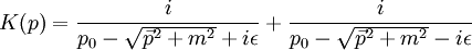
![S[\phi] \,](images/math/7/5/7/757305e5a5c916d1c50a851df3733788.png) where the field
where the field  is itself a function of space and time, and the square brackets are a reminder that the action depends on all the field's values everywhere, not just some particular value. In principle, one integrates Feynman's amplitude over the class of all possible combinations of values that the field could have anywhere in space-time.
 of field configurations (which only depends locally on the fields), then the time ordered vacuum expectation value of polynomially bounded functional F, <F>, is given by
![\left\langle F\right\rangle=\frac{\int \mathcal{D}\phi F[\phi]e^{i\mathcal{S}[\phi]}}{\int\mathcal{D}\phi e^{i\mathcal{S}[\phi]}}](images/math/d/0/8/d080231c5a3ebd0967b86a2c94a58d97.png)
 here is a concise way to represent the infinite-dimensional integral over all possible field configurations on all of space-time. As stated above, we put the unadorned path integral in the denominator to normalize everything properly.
![\frac{\delta \mathcal{S}[\phi]}{\delta \phi}=0](images/math/a/4/d/a4da78df67facd63f6bbb17aca29a45a.png) (the left-hand side is a functional derivative; the equation means that the action is stationary under small changes in the field configuration). The quantum analogues of these equations are called the Schwinger-Dyson equations.
(the left-hand side is a functional derivative; the equation means that the action is stationary under small changes in the field configuration). The quantum analogues of these equations are called the Schwinger-Dyson equations.
 turns out to be translationally invariant (we'll assume this for the rest of this article, although this does not hold for, let's say nonlinear sigma models) and if we assume that after a
 ![e^{i\mathcal{S}[\phi]},](images/math/4/e/9/4e92581abddcf745494dc90aa7b890ba.png)
![e^{-H[\phi]}\,](images/math/0/4/6/0466911124144e947752b1b5069b5359.png)
![\left\langle \frac{\delta F[\phi]}{\delta \phi} \right\rangle = -i \left\langle F[\phi]\frac{\delta \mathcal{S}[\phi]}{\delta\phi} \right\rangle](images/math/2/3/f/23fcf1fecd6d773639803a3c631a0679.png)
![Z[J]=\int \mathcal{D}\phi e^{i(\mathcal{S}[\phi] + \left\langle J,\phi \right\rangle)}.](images/math/e/d/2/ed2b182edd8a83360f3f258c0c895a44.png)
![\frac{\delta^n Z}{\delta J(x_1) \cdots \delta J(x_n)}[J] = i^n \, Z[J] \, {\left\langle \phi(x_1)\cdots \phi(x_n)\right\rangle}_J](images/math/d/8/8/d88a903e8ac2e9610910e945bd648652.png)
![Z^{,i_1\dots i_n}[J]=i^n Z[J] {\left \langle \phi^{i_1}\cdots \phi^{i_n}\right\rangle}_J](images/math/0/b/3/0b3e89638ea274fd195c91dfae0311dd.png)
![{\left\langle F \right\rangle}_J=\frac{\int \mathcal{D}\phi F[\phi]e^{i(\mathcal{S}[\phi] + \left\langle J,\phi \right\rangle)}}{\int\mathcal{D}\phi e^{i(\mathcal{S}[\phi] + \left\langle J,\phi \right\rangle)}}.](images/math/4/2/f/42f37a80fd916e7de98003833af046b7.png)
![\mathcal{D}\phi e^{i\mathcal{S}[\phi]}](images/math/3/a/d/3add188359239f008f7c7d1c96610ec4.png) is viewed as a functional distribution (this shouldn't be taken too literally as an interpretation of QFT, unlike its Wick rotated
is viewed as a functional distribution (this shouldn't be taken too literally as an interpretation of QFT, unlike its Wick rotated 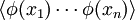 are its moments and Z is its Fourier transform.
![F[\phi]=\frac{\partial^{k_1}}{\partial x_1^{k_1}}\phi(x_1)\cdots \frac{\partial^{k_n}}{\partial x_n^{k_n}}\phi(x_n)](images/math/d/8/5/d852e4b9cfd279c320d01bf450e6f1b4.png)
![F\left[-i\frac{\delta}{\delta J}\right] G[J] = (-i)^n \frac{\partial^{k_1}}{\partial x_1^{k_1}}\frac{\delta}{\delta J(x_1)} \cdots \frac{\partial^{k_n}}{\partial x_n^{k_n}}\frac{\delta}{\delta J(x_n)} G[J].](images/math/e/2/9/e29d2540e9e179a95b3b2ac2b4d5ae6a.png)
![\frac{\delta \mathcal{S}}{\delta \phi(x)}\left[-i \frac{\delta}{\delta J}\right]Z[J]+J(x)Z[J]=0](images/math/8/6/c/86c3c50832e40dce6cb26cfc38428474.png)
![\mathcal{S}_{,i}[-i\partial]Z+J_i Z=0.](images/math/b/b/8/bb83ee361101d4ca58d3a48029e2d306.png)
![M\left[\phi\right]\,\mathcal{D}\phi](images/math/3/9/6/396bacaa9c73c517ddf82cd90c0f082f.png) where M is a functional and
where M is a functional and 
![\int D[x]e^{-\mathcal{S}[x]/\hbar}=-A[x]\sum_{n=0}^{\infty}(\hbar)^{n+1}\delta^{n} e^{-J/\hbar}](images/math/2/b/d/2bd8771527dec96411e1631acabddc52.png)
![A[x]=\exp\left({1/\hbar}\int X(t)\,\mathrm{d}t\right).](images/math/f/5/7/f5706c34706cae6afe162a5698655cb0.png)
![Q[\mathcal{L}(x)]=\partial_\mu f^\mu (x)](images/math/2/5/2/2526ee343153e827b72fab1755c9dafc.png) for some function f where f only depends locally on φ (and possibly the spacetime position).
for some function f where f only depends locally on φ (and possibly the spacetime position).
![\int \mathcal{D}\phi Q[F][\phi]=0](images/math/8/3/9/83955a2161dd30a597defe9bf0e8d820.png) for any polynomially bounded functional F. This property is called the invariance of the measure. And this does not hold in general. See anomaly (physics) for more details.
for any polynomially bounded functional F. This property is called the invariance of the measure. And this does not hold in general. See anomaly (physics) for more details.
![\int \mathcal{D}\phi\, Q[F e^{iS}][\phi]=0,](images/math/7/c/c/7cc0fe276e23d3f18e4ed833b4caab03.png)
![\left\langle Q[F]\right\rangle +i\left\langle F\int_{\partial V} f^\mu ds_\mu\right\rangle=0](images/math/b/3/a/b3a2ac79cdfbe4fedb6b375efe9e7465.png)
![q(x)[\phi(y)] = \delta^{(d)}(X-y)Q[\phi(y)] \,](images/math/7/a/a/7aa36978d066a8d6614704206edbfd0e.png)
![q(x)[S]=\partial_\mu j^\mu (x) \,](images/math/5/9/1/591281c46c1ecd2593a5922ccad51c08.png)
![j^{\mu}(x)=f^\mu(x)-\frac{\partial}{\partial (\partial_\mu \phi)}\mathcal{L}(x) Q[\phi] \,](images/math/8/d/0/8d0ee9f64813c047f0d20b2f993696cf.png)
![\int \mathcal{D}\phi\, q(x)[F][\phi]=0.](images/math/5/3/c/53cbf084b75b3a913c545b585496b222.png)
![\left\langle q(x)[F] \right\rangle +i\left\langle F q(x)[S]\right\rangle=\left\langle q(x)[F]\right\rangle +i\left\langle F\partial_\mu j^\mu(x)\right\rangle=0.](images/math/c/c/2/cc272281e5e228646e8d54e7bb1da28c.png)
![q(x)[S][-i \frac{\delta}{\delta J}]Z[J]+J(x)Q[\phi(x)][-i \frac{\delta}{\delta J}]Z[J]=\partial_\mu j^\mu(x)[-i \frac{\delta}{\delta J}]Z[J]+J(x)Q[\phi(x)][-i \frac{\delta}{\delta J}]Z[J]=0.](images/math/b/a/c/bac36f20df1cd43fa16a86fb45d95980.png)
![\left\langle Q[F]\right\rangle =0.](images/math/3/f/3/3f36b29b3ddc33b7395638cd029aed5c.png)
![\int d^dx\, J(x)Q[\phi(x)][-i \frac{\delta}{\delta J}]Z[J]=0.](images/math/1/5/7/157fcb2d1796115736089a8db6ebb38e.png)


