To use all functions of this page, please activate cookies in your browser.
My watch list
my.chemeurope.com
my.chemeurope.com
With an accout for my.chemeurope.com you can always see everything at a glance – and you can configure your own website and individual newsletter.
- My watch list
- My saved searches
- My saved topics
- My newsletter
Perturbation theory
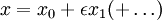
Perturbation theory comprises mathematical methods that are used to find an approximate solution to a problem which cannot be solved exactly, by starting from the exact solution of a related problem. Perturbation theory is applicable if the problem at hand can be formulated by adding a "small" term to the mathematical description of the exactly solvable problem. Perturbation theory leads to an expression for the desired solution in terms of a power series in some "small" parameter that quantifies the deviation from the exactly solvable problem. The leading term in this power series is the solution of the exactly solvable problem, while further terms describe the deviation in the solution, due to the deviation from the initial problem. Formally, we have for the approximation to the full solution A, a series in the small parameter (here called ε), like the following: In this example, A0 would be the known solution to the exactly solvable initial problem and Additional recommended knowledge
ExamplesExamples for the "mathematical description" are: an algebraic equation, a differential equation (e.g., the equations of motion in celestial mechanics or a wave equation), a free energy (in statistical mechanics), a Hamiltonian operator (in quantum mechanics). Examples for the kind of solution to be found perturbatively: the solution of the equation (e.g., the trajectory of a particle), the statistical average of some physical quantity (e.g., average magnetization), the ground state energy of a quantum mechanical problem. Examples for the exactly solvable problems to start with: Linear equations, including linear equations of motion (harmonic oscillator, linear wave equation), statistical or quantum-mechanical systems of non-interacting particles (or in general, Hamiltonians or free energies containing only terms quadratic in all degrees of freedom). Examples of "perturbations" to deal with: Nonlinear contributions to the equations of motion, interactions between particles, terms of higher powers in the Hamiltonian/Free Energy. For physical problems involving interactions between particles, the terms of the perturbation series may be displayed (and manipulated) using Feynman diagrams. HistoryPerturbation theory has its roots in 17th century celestial mechanics, where the theory of epicycles was used to make small corrections to the predicted paths of planets.[citation needed] Curiously, it was the need for more and more epicycles that eventually led to the 16th century Copernican revolution in the understanding of planetary orbits. The development of basic perturbation theory for differential equations was fairly complete by the middle of the 19th century. It was at that time that Charles-Eugène Delaunay was studying the perturbative expansion for the Earth-Moon-Sun system, and discovered the so-called "problem of small denominators". Here, the denominator appearing in the n'th term of the perturbative expansion could become arbitrarily small, causing the n'th correction to be as large or larger than the first-order correction. At the turn of the 20th century, this problem led Henri Poincare to make one of the first deductions of the existence of chaos, or what is prosaically called the "butterfly effect": that even a very small perturbation can have a very large effect on a system. Perturbation theory saw a particularly dramatic expansion and evolution with the arrival of quantum mechanics. Although perturbation theory was used in the semi-classical theory of the Bohr atom, the calculations were monstrously complicated, and subject to somewhat ambiguous interpretation. The discovery of Heisenberg's matrix mechanics allowed a vast simplification of the application of perturbation theory. Notable examples are the Stark effect and the Zeeman effect, which have a simple enough theory to be included in standard undergraduate textbooks in quantum mechanics. Other early applications include the fine structure and the hyperfine structure in the hydrogen atom. In modern times, perturbation theory underlies much of quantum chemistry and quantum field theory. In chemistry, perturbation theory was used to obtain the first solutions for the helium atom. In the middle of the 20'th century, Richard Feynman realized that the perturbative expansion could be given a dramatic and beautiful graphical representation in terms of what are now called Feynman diagrams. Although originally applied only in quantum field theory, such diagrams now find increasing use in any area where perturbative expansions are studied. A partial resolution of the small-divisor problem was given by the statement of the KAM theorem in 1954. Developed by Andrey Kolmogorov, Vladimir Arnold and Jurgen Moser, this theorem stated the conditions under which a system of partial differential equations will have only mildly chaotic behaviour under small perturbations. In the late 20th century, broad dissatisfaction with perturbation theory in the quantum physics community, including not only the difficulty of going beyond second order in the expansion, but also questions about whether the perturbative expansion is even convergent, has led to a strong interest in the area of non-perturbative analysis, that is, the study of exactly solvable models. The prototypical model is the KdV equation, a highly non-linear equation for which the interesting solutions, the solitons, cannot be reached by perturbation theory, even if the perturbations were carried out to infinite order. Much of the theoretical work in non-perturbative analysis goes under the name of quantum groups and non-commutative geometry. Perturbation ordersThe standard exposition of perturbation theory is given in terms the order to which the perturbation is carried out: first order perturbation theory or second order perturbation theory, and whether the perturbed states are degenerate (that is, singular), in which case extra care must be taken, and the theory is slightly more difficult.
First-order non-singular perturbation theoryThis section develops, in simplified terms, the general theory for the perturbative solution to a differential equation to the first order. In order to keep the exposition simple, a crucial assumption is made: that the solutions to the unperturbed system are not degenerate, so that the perturbation series can be inverted. There are ways of dealing with the degenerate (or "singular") case; these require extra care. Suppose one wants to solve a differential equation of the form
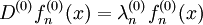
where D is some specific differential operator, and λ is an eigenvalue. Many problems involving ordinary or partial differential equations can be cast in this form. It is presumed that the differential operator can be written in the form
where ε is presumed to be small, and that furthermore, the complete set of solutions for D(0) are known. That is, one has a set of solutions
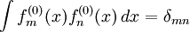
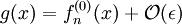
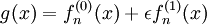
Furthermore, one assumes that the set of solutions with δmn the Kronecker delta function. To zeroth order, one expects that the solutions g(x) are then somehow "close" to one of the unperturbed solutions and
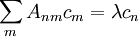
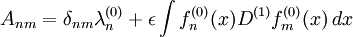
where with all of the constants This can be trivially re-written as a simple linear algebra problem of finding the eigenvalue of a matrix, where where the matrix elements Anm are given by Rather than solving this full matrix equation, one notes that, of all the cm in the linear equation, only one, namely cn, is not small. Thus, to the first order in ε, the linear equation may be solved trivially as since all of the other terms in the linear equation are of order The function g(x) to first order is obtained through similar reasoning. Substituting so that gives an equation for to give which gives the exact solution to the perturbed differential equation to the first order in the perturbation ε. Several important observations can be made about the form of this solution. First, the sum over functions with differences of eigenvalues in the denominator resembles the resolvent in Fredholm theory. This is no accident; the resolvent acts essentially as a kind of Green's function or propagator, passing the perturbation along. Higher order perturbations resemble this form, with an additional sum over a resolvent appearing at each order. The form of this solution is sufficient to illustrate the idea behind the small-divisor problem. If, for whatever reason, two eigenvalues are close so that difference Curiously, the situation is not at all bad if two or more eigenvalues are exactly equal. This case is referred to as singular or degenerate perturbation theory. The degeneracy of eigenvalues indicates that the unperturbed system has some sort of symmetry, and that the generators of the symmetry commute with the unperturbed differential equation. Typically, the perturbing term does not possess the symmetry; one says the perturbation lifts or breaks the degeneracy. In this case, the perturbation can still be performed; however, one must be careful to work in a basis for the unperturbed states so that these map one-to-one to the perturbed states, rather than being a mixture. Example of second-order singular perturbation theoryConsider the following equation for the unknown variable x:
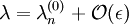
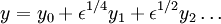
For the initial problem with ε = 0, the solution is x0 = 1. For small ε the lowest order approximation may be found by inserting the ansatz into the equation and demanding the equation to be fulfilled up to terms that involve powers of ε higher than the first. This yields x1 = 1. In the same way, the higher orders may be found. However, even in this simple example it may be observed that for (arbitrarily) small ε > 0 there are four other solutions to the equation (with very large magnitude). The reason we don't find these solutions in the above perturbation method is because these solutions diverge when The four additional solutions can be found using the methods of singular perturbation theory. In this case this works as follows. Since the four solutions diverge at ε = 0, it makes sense to rescale x. We put
such that in terms of y the solutions stay finite. This means that we need to choose the exponent ν to match the rate at which the solutions diverge. In terms of y the equation reads:
The 'right' value for ν is obtained when the exponent of ε in the prefactor of the term proportional to y is equal to the exponent of ε in the prefactor of the term proportional to y5, i.e. when ν = 1 / 4. This is called 'significant degeneration'. If we choose ν larger, then the four solutions will collapse to zero in terms of y and they will become degenerate with the solution we found above. If we choose ν smaller, then the four solutions will still diverge to infinity. Putting ν = 1 / 4 in the above equation yields:
This equation can be solved using ordinary perturbation theory in the same way as regular expansion for x was obtained. Since the expansion parameter is now ε1 / 4 we put: There are 5 solutions for y0: 0, 1, -1, i and -i. We must disregard the solution y = 0. The case y = 0 corresponds to the original regular solution which appears to be at zero for ε = 0, because in the limit
CommentaryBoth regular and singular perturbation theory are frequently used in physics and engineering. Regular perturbation theory may only be used to find those solutions of a problem that evolve smoothly out of the initial solution when changing the parameter (that are "adiabatically connected" to the initial solution). A well known example from physics where regular perturbation theory fails is in fluid dynamics when one treats the viscosity as a small parameter. Close to a boundary, the fluid velocity goes to zero, even for very small viscosity (the no-slip condition). For zero viscosity, it is not possible to impose this boundary condition and a regular perturbative expansion amounts to an expansion about an unrealistic physical solution. Singular perturbation theory can, however, be applied here and this amounts to 'zooming in' at the boundaries (using the method of matched asymptotic expansions). Perturbation theory can fail when the system can go to a different "phase" of matter, with a qualitatively different behaviour that cannot be understood by perturbation theory (e.g., a solid crystal melting into a liquid). In some cases this failure manifests itself by divergent behavior of the perturbation series. Such divergent series can sometimes be resummed using techniques such as Borel resummation. Perturbation techniques can be also used to find approximate solutions to non-linear differential equations. Examples of techniques used to find approximate solutions to these types of problems are the Lindstedt-Poincaré technique, the method of harmonic balancing, and the method of multiple time scales. There is absolutely no guarantee perturbative methods would result in a convergent solution. In fact, asymptotic series are the norm. Perturbation theory in chemistryMany of the ab initio quantum chemistry methods use perturbation theory directly or are closely related methods. Møller-Plesset perturbation theory uses the difference between the Hartree-Fock Hamiltonian and the exact non-relativistic Hamiltonian as the perturbation. The zero order energy is the sum of orbital energies. The first-order energy is the Hartree-Fock energy and electron correlation is included at second-order or higher. Calculations to second, third or forth order are very common and the code is included in most ab initio quantum chemistry programs. A related but more accurate method is the coupled cluster method. See also
|
|
| This article is licensed under the GNU Free Documentation License. It uses material from the Wikipedia article "Perturbation_theory". A list of authors is available in Wikipedia. |

 represent the "higher orders" which are found iteratively by some systematic procedure. For small


 , labelled by some arbitrary index n, such that
 .
.
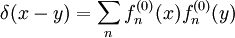
 form an orthonormal set:
 .
.
 denotes the relative size, in big-O notation. To solve this problem, one assumes that the solution
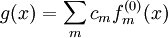
 except for n, where
  . Substituting this last expansion into the differential equation, taking the inner product of the result with
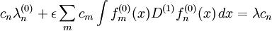
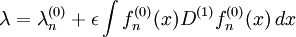
 . The above gives the solution of the eigenvalue to first order in perturbation theory.

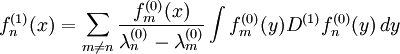
 . It may be solved integrating with the partition of unity
 become small, the corresponding term in the sum will become disproportionately large. In particular, if this happens in higher-order terms, the high order perturbation may become as large or larger in magnitude than the first-order perturbation. Such a situation calls into question the validity of doing a perturbation to begin with. This can be understood to be a fairly catastrophic situation; it is frequently encountered in chaotic dynamical systems, and requires the development of techniques other than perturbation theory to solve the problem.
 while the ansatz assumes regular behavior in this limit.
![x = \epsilon^{-1/4}\left[y_0 - 1/4\epsilon^{1/4} +\ldots\right]](images/math/7/c/7/7c7375a98659728d5aa92a5a31900a82.png)


