To use all functions of this page, please activate cookies in your browser.
My watch list
my.chemeurope.com
my.chemeurope.com
With an accout for my.chemeurope.com you can always see everything at a glance – and you can configure your own website and individual newsletter.
- My watch list
- My saved searches
- My saved topics
- My newsletter
Quantum statistical mechanicsQuantum statistical mechanics is the study of statistical ensembles of quantum mechanical systems. A statistical ensemble is described by a density operator S, which is a non-negative, self-adjoint, trace-class operator of trace 1 on the Hilbert space H describing the quantum system. This can be shown under various mathematical formalisms for quantum mechanics. One such formalism is provided by quantum logic. Additional recommended knowledge
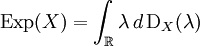
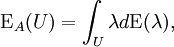
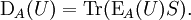
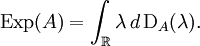
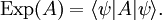
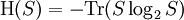
ExpectationFrom classical probability theory, we know that the expectation of a random variable X is completely determined by its distribution DX by assuming, of course, that the random variable is integrable or that the random variable is non-negative. Similarly, let A be an observable of a quantum mechanical system. A is given by a densely defined self-adjoint operator on H. The spectral measure of A defined by uniquely determines A and conversely, is uniquely determined by A. EA is a boolean homomorphism from the Borel subsets of R into the lattice Q of self-adjoint projections of H. In analogy with probability theory, given a state S, we introduce the distribution of A under S which is the probability measure defined on the Borel subsets of R by Similarly, the expected value of A is defined in terms of the probability distribution DA by Note that this expectation is relative to the mixed state S which is used in the definition of DA. Remark. For technical reasons, one needs to consider separately the positive and negative parts of A defined by the Borel functional calculus for unbounded operators. One can easily show: Note that if S is a pure state corresponding to the vector ψ, Von Neumann entropyOf particular significance for describing randomness of a state is the von Neumann entropy of S formally defined by
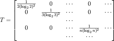
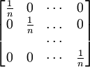
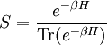
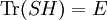
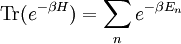
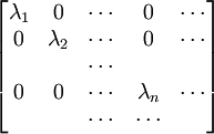
Actually, the operator S log2 S is not necessarily trace-class. However, if S is a non-negative self-adjoint operator not of trace class we define Tr(S) = +∞. Also note that any density operator S can be diagonalized, that it can be represented in some orthonormal basis by a (possibly infinite) matrix of the form and we define The convention is that Remark. It is indeed possible that H(S) = +∞ for some density operator S. In fact T be the diagonal matrix T is non-negative trace class and one can show T log2 T is not trace-class. Theorem. Entropy is a unitary invariant. In analogy with classical entropy (notice the similarity in the definitions), H(S) measures the amount of randomness in the state S. The more dispersed the eigenvalues are, the larger the system entropy. For a system in which the space H is finite-dimensional, entropy is maximized for the states S which in diagonal form have the representation For such an S, H(S) = log2 n. The state S is called the maximally mixed state. Recall that a pure state is one of the form for ψ a vector of norm 1. Theorem. H(S) = 0 if and only if S is a pure state. For S is a pure state if and only if its diagonal form has exactly one non-zero entry which is a 1. Entropy can be used as a measure of quantum entanglement. Gibbs canonical ensembleConsider an ensemble of systems described by a Hamiltonian H with average energy E. If H has pure-point spectrum and the eigenvalues En of H go to + ∞ sufficiently fast, e-r H will be a non-negative trace-class operator for every positive r. The Gibbs canonical ensemble is described by the state where β is such that the ensemble average of energy satisfies ,and is the quantum mechanical version of the canonical partition function. The probability that a system chosen at random from the ensemble will be in a state corresponding to energy eigenvalue Em is Under certain conditions, the Gibbs canonical ensemble maximizes the von Neumann entropy of the state subject to the energy conservation requirement. References
Categories: Statistical mechanics | Quantum mechanical entropy |
|
| This article is licensed under the GNU Free Documentation License. It uses material from the Wikipedia article "Quantum_statistical_mechanics". A list of authors is available in Wikipedia. |


 .
.

 , since an event with probability zero should not contribute to the entropy. This value is an extended real number (that is in [0, ∞]) and this is clearly a unitary invariant of S.