To use all functions of this page, please activate cookies in your browser.
My watch list
my.chemeurope.com
my.chemeurope.com
With an accout for my.chemeurope.com you can always see everything at a glance – and you can configure your own website and individual newsletter.
- My watch list
- My saved searches
- My saved topics
- My newsletter
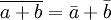
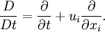
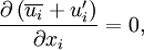
Reynolds stressesIn fluid dynamics, the Reynolds stresses (or, the Reynolds stress tensor) is the stress tensor in a fluid due to the random turbulent fluctuations in fluid momentum. The stress is obtained from an average (typically in some loosely defined fashion) over these fluctuations. Additional recommended knowledgeTo illustrate, here we use Cartesian vector index notation. For simplicity, consider an incompressible fluid: Given the fluid velocity ui as a function of position and time, write the average fluid velocity as The conventional ensemble rules of averaging are that One splits the Euler equations or the Navier-Stokes equations into an average and a fluctuating part. One finds that upon averaging the fluid equations, a stress on the right hand side appears of the form The divergence of this stress is the force density on the fluid due to the turbulent fluctuations. For instance, for an incompressible, viscous, Newtonian fluid, the continuity and momentum equations can be written as
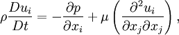
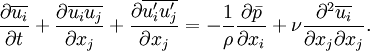
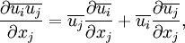
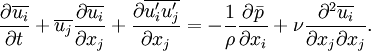
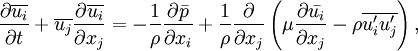
and where D / Dt is the Lagrangian derivative, Defining the flow variables above with a time-averaged component and a fluctuating component, the continuity and momentum equations become and Examining one of the terms on the left hand side of the momentum equation, it is seen that where the last term on the right hand side vanishes as a result of the continuity equation. Accordingly, the momentum equation becomes Now the continuity and momentum equations will be averaged. The ensemble rules of averaging need to be employed, keeping in mind that the average of products of fluctuating quantities will not in general vanish. After averaging, the continuity and momentum equations become and Dividing both sides of the momentum equation by ρ yields Using the chain rule on one of the terms of the left hand side, it is revealed that where the last term on the right hand side vanishes as a result of the averaged continuity equation. The averaged momentum equation now becomes This equation can be rearranged to arrive at a well-known form, where the Reynolds stresses, The question then is, what is the value of the Reynolds stress? This has been the subject of intense modeling and interest, for roughly the past century. The problem is recognized as a closure problem, akin to the problem of closure in the BBGKY hierarchy. A transport equation for the Reynolds stress may be found by taking the outer product of the fluid equations for the fluctuating velocity, with itself. One finds that the transport equation for the Reynolds stress includes terms with higher-order correlations (specifically, the triple correlation It should also be noted that the theory of the Reynolds stress is quite analogous to the kinetic theory of gases, and indeed the stress tensor in a fluid at a point may be seen to be the ensemble average of the stress due to the thermal velocities of molecules at a given point in a fluid. Thus, by analogy, the Reynolds stress is sometimes thought of as consisting of an isotropic pressure part, termed the turbulent pressure, and an off-diagonal part which may be thought of as an effective turbulent viscosity. In fact, while much effort has been expended in developing good models for the Reynolds stress in a fluid, as a practical matter, when solving the fluid equations using computational fluid dynamics, often the simplest turbulence models prove the most effective. One class of models, closely related to the concept of turbulent viscosity, is the so-called K − ε model(s), based upon coupled transport equations for the turbulent energy density K (similar to the turbulent pressure, i.e. the trace of the Reynolds stress) and the turbulent dissipation rate ε. Typically, the average is formally defined as an ensemble average as in statistical ensemble theory. However, as a practical matter, the average may also be thought of as a spatial average over some lengthscale, or a temporal average. Note that, while formally the connection between such averages is justified in equilibrium statistical mechanics by the ergodic theorem, the statistical mechanics of hydrodynamic turbulence is currently far from understood. In fact, the Reynolds stress at any given point in a turbulent fluid is somewhat subject to interpretation, depending upon how one defines the average. |
| This article is licensed under the GNU Free Documentation License. It uses material from the Wikipedia article "Reynolds_stresses". A list of authors is available in Wikipedia. |


 , and the velocity fluctuation is
 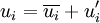 .
.


 . This is the Reynolds stress, conventionally written
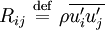
 ,
,
![\rho \left[ \frac{\partial \left( \overline{u_i} + u_i' \right)}{\partial t} + \left( \overline{u_j} + u_j' \right) \frac{\partial \left( \overline{u_i} + u_i' \right)}{\partial x_j} \right] = -\frac{\partial \left( \bar{p} + p' \right) }{\partial x_i} + \mu \left[ \frac{\partial^2 \left( \overline{u_i} + u_i' \right)}{\partial x_j \partial x_j} \right].](images/math/a/c/2/ac29573a3107049ffc0ebc7e1b2f85eb.png)

![\rho \left[ \frac{\partial \left( \overline{u_i} + u_i' \right)}{\partial t} + \frac{\partial \left( \overline{u_i} + u_i' \right) \left( \overline{u_j} + u_j' \right) }{\partial x_j} \right] = -\frac{\partial \left( \bar{p} + p' \right) }{\partial x_i} + \mu \left[ \frac{\partial^2 \left( \overline{u_i} + u_i' \right)}{\partial x_j \partial x_j} \right].](images/math/2/b/2/2b2c2d3584d9fd0c6771158d35f149d5.png)

![\rho \left[ \frac{\partial \overline{u_i}}{\partial t} + \frac{\partial \overline{u_i} \overline{u_j}}{\partial x_j} + \frac{\partial \overline{u_i'} \overline{u_j'}}{\partial x_j} \right] = -\frac{\partial \bar{p}}{\partial x_i} + \mu \frac{\partial^2 \overline{u_i}}{\partial x_j \partial x_j}.](images/math/b/f/3/bf3f83fef6b1dbc0aa5a34b83f008cb2.png)
 , are collected with the traditional normal and shear stress terms,
  .
.
 ) as well as correlations with pressure fluctuations (i.e. momentum carried by sound waves). A common solution is to model these terms by simple ad-hoc prescriptions.


