To use all functions of this page, please activate cookies in your browser.
My watch list
my.chemeurope.com
my.chemeurope.com
With an accout for my.chemeurope.com you can always see everything at a glance – and you can configure your own website and individual newsletter.
- My watch list
- My saved searches
- My saved topics
- My newsletter
Theory of tidesThe theory of tides is the application of continuum mechanics to interpret and predict the tidal deformations of planetary and satellite bodies and their atmospheres and oceans, under the gravitational loading of another astronomical body or bodies. It commonly refers to the fluid dynamic motions for the Earth's oceans. Additional recommended knowledge
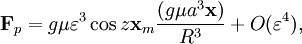
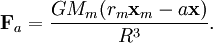
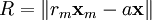
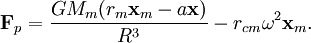
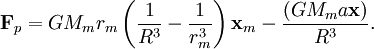
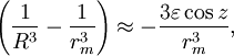
Tidal physicsTidal forcingThe forces discussed here apply to body (Earth tides), oceanic and atmospheric tides. Atmospheric tides on Earth, however, tend to be dominated by forcing due to solar heating. On the planet (or satellite) experiencing tidal motion consider a point at latitude φ and longitude λ at distance a from the center of mass, then point can written in cartesian coordinates as Let δ be the declination and α be the right ascension of the deforming body, the Moon for example, then the vector direction is and rm be the orbital distance between the center of masses and Mm the mass of the body. Then the force on the point is where where rcm is the distance between the center of mass for the orbit and planet and M is the planetary mass. Consider the point in the reference fixed without rotation, but translating at a fixed translation with respect to the center of mass of the planet. The body's centripetal force acts on the point so that the total force is Substituting for center of mass acceleration, and reordering In ocean tidal forcing, the radial force is not significant, the next step is to rewrite the where if ε is small. If particle is on the surface of the planet then the local gravity is
which is a small fraction of g. Note also that force is attractive toward the Moon when the z < π / 2 and repulsive when z > π / 2. This can also be used to derive a tidal potential. Laplace tidal equationsLaplace summarized the work to his time with a single set of linear partial differential equations simplified from the fluid dynamic equations, but can also be derived via Lagranges equation from energy integrals. It summarizes tidal flow as a barotropic two-dimensional sheet flow, where Coriolis effects are introduced a fictious lateral force. Thomson rewote Laplace's momentum terms using the curl to find an equation for vorticity. Under certain conditions this can be further rewritten as a conservation of vorticity. Tidal analysis and predictionHarmonic analysisThere are about 62 constituents that could be used, but many less are needed to predict tides accurately. Tidal constituentsExample amplitudes from Eastport, ME; Biloxi, MS; San Juan, PR; Kodiak, AK; San Francisco, CA; and Hilo HI;. Categories: Continuum mechanics | Fluid dynamics | Fluid mechanics |
|||
| This article is licensed under the GNU Free Documentation License. It uses material from the Wikipedia article "Theory_of_tides". A list of authors is available in Wikipedia. |


 where
where


 For a circular orbit the angular momentum
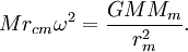
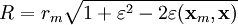
 coefficient. Let
  then
then
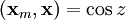 is the inner product determining the angle z of the deforming body or Moon from the zenith. This means that
 and
set
and
set