My watch list

Green's function

In mathematics, Green's function is a type of function used to solve inhomogeneous differential equations subject to boundary conditions. The term is used in physics, specifically in quantum field theory and statistical field theory, to refer to various types of correlation functions, even those that do not fit the mathematical definition; for this sense, see Correlation function (quantum field theory) and Green's function (many-body theory).

Green's function is named after the British mathematician George Green, who first developed the concept in the 1830s.

Additional recommended knowledge

What is the Correct Way to Check Repeatability in Balances?

How to ensure accurate weighing results every day?

Daily Sensitivity Test

1 Definition and uses
2 Motivation
3 Green's function for solving inhomogeneous boundary value problems
- 3.1 Working frame
- 3.2 Theorem
4 Finding Green's functions
- 4.1 Eigenvalue expansions
5 Green's function for the Laplacian
6 Example
7 Further examples
8 See also
9 References

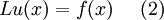
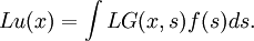
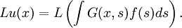
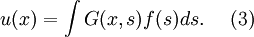
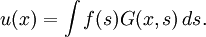
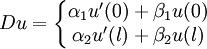
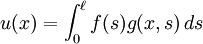
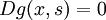
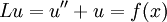
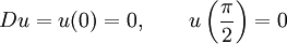
Definition and uses

Technically, a Green's function, G(x, s), of a linear operator L acting on distributions over a manifold M, at a point x₀, is any solution of

$L G (x,s) = \delta(x-s) \ \ \ \ \ (1)$

where $δ$ is the Dirac delta function. This technique can be used to solve differential equations of the form;

$L u(x) = f(x) \ \ \ \ (2)$

If the kernel of L is nontrivial, then the Green's function is not unique. However, in practice, some combination of symmetry, boundary conditions and/or other externally imposed criteria would give us a unique Green's function. Also, Green's functions in general are distributions, not necessarily proper functions.

Green's functions are also a useful tool in condensed matter theory, where they allow the resolution of the diffusion equation - and in quantum mechanics, where the Green's function of the Hamiltonian is a key concept, with important links to the concept of density of states. The Green's functions used in those two domains are highly similar, due to the analogy in the mathematical structure of the diffusion equation and Schrödinger equation.

Motivation

Loosely speaking, if such a function G can be found for the operator L, then if we multiply the equation (1) for the Green's function by f(s), and then perform an integration in the s variable, we obtain;

$\int L G(x,s) f(s) ds = \int \delta(x-s)f(s) ds = f(x).$

The right hand side is now given by the equation (2) to be equal to Lu(x), thus;

$Lu(x) = \int L G(x,s) f(s) ds.$

Because the operator L is linear and acts on the variable x alone (not on the variable of integration s), we can take the operator L outside of the integration on the right hand side obtaining;

$Lu(x) = L\left(\int G(x,s) f(s) ds\right).$

And this implies;

$u(x) = \int G(x,s) f(s) ds . \ \ \ \ (3)$

Thus, we can obtain the function u(x) through knowledge of the Green's function in equation (1), and the source term on the right hand side in equation (2). This process has resulted from the linearity of the operator L.

In other words, the solution of equation (2), u(x), can be determined by the integration given in equation (3). Although f(x) is known, this integration cannot be performed unless G is also known. The problem now lies in finding the Green's function G that satisfies equation (1).

Not every operator L admits a Green's function. A Green's function can also be thought of as a right inverse of L. Aside from the difficulties of finding a Green's functions for a particular operator, the integral in equation (3), may be quite difficult to perform. However the method gives a theoretically exact result.

Convolving with a Green's function gives solutions to inhomogeneous differential-integral equations, most commonly a Sturm-Liouville problem. If G is the Green's function of an operator L, then the solution for u of the equation Lu = f is given by

$u(x) = \int{ f(s) G(x,s) \, ds}.$

This can be thought of as an expansion of f according to a Dirac delta function basis (projecting f over δ(x − s)) and a superposition of the solution on each projection. Such an integral is known as a Fredholm integral equation, the study of which constitutes Fredholm theory.

Green's function for solving inhomogeneous boundary value problems

The primary use of Green's functions in mathematics is to solve inhomogeneous boundary value problems. In modern theoretical physics, Green's functions are also usually used as propagators in Feynman diagrams (and the phrase "Green's function" is often used for any correlation function).

Working frame

Let $L$ be the Sturm-Liouville operator, a linear differential operator of the form

$L = {d \over dx}\left[ p(x) {d \over dx} \right] + q(x)$

and let D be the boundary conditions operator

$Du = \left\{\begin{matrix} \alpha _1 u'(0) + \beta _1 u(0) \\ \alpha _2 u'(l) + \beta _2 u(l) \end{matrix}\right.$

Let $f (x)$ be a continuous function in $[0, l]$ . We shall also suppose that the problem

$\begin{matrix}Lu = f \\ Du = 0 \end{matrix}$

is regular, i.e. only the trivial solution exists for the homogeneous problem.

Theorem

Then there is one and only one solution u(x) which satisfies

$\begin{matrix}Lu = f \\ Du = 0 \end{matrix}$

and it is given by

$u(x) = \int_0^\ell f(s) g(x,s) \, ds$

where g(x,s) is Green's function and satisfies the following demands:

g(x,s) is continuous in x and s.
For $x \ne s$ , $L g ( x, s ) = 0 \,$ .
For $s \ne 0, l$ , $D g ( x, s ) = 0 \,$ .
Derivative "jump": $g ' ( s_{ + 0}, s ) - g ' (s_{ - 0}, s ) = 1 / p(s). \,$
Symmetry: g(x, s) = g(s, x).

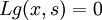
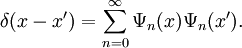
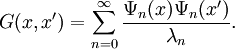
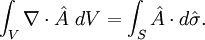
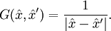
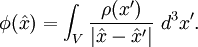
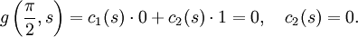
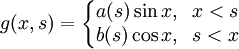
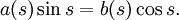
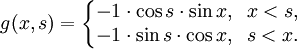
Finding Green's functions

Eigenvalue expansions

If a differential operator L admits a set of eigenvectors $Ψ n (x)$ (i.e. a set of functions $Ψ n (x)$ and scalars $λ n$ such that $L Ψ n = λ n Ψ n)$ ) that are complete, then we can construct a Green's function from these eigenvectors and eigenvalues.

By complete, we mean that the set of functions : $Ψ n (x)$ satisfies the following completeness relation:

$\delta(x - x') = \sum_{n=0}^\infty \Psi_n(x) \Psi_n(x').$

We can prove the following:

$G(x, x') = \sum_{n=0}^\infty \frac{\Psi_n(x) \Psi_n(x')}{\lambda_n}.$

Now consider acting on this on each side with the operator L. We end up with the completeness relation, which was assumed true.

The general study of the Green's function written in the above form, and its relationship to the function spaces formed by the eigenvectors, is known as Fredholm theory.

Green's function for the Laplacian

Green's functions for linear differential operators involving the Laplacian may be readily put to use using the second of Green's identities.

To derive Green's theorem, begin with the divergence theorem (otherwise known as Gauss's law):

$\int_V \nabla \cdot \hat A\ dV = \int_S \hat A \cdot d\hat\sigma.$

Let $A = \phi\nabla\psi - \psi\nabla\phi$ and substitute into Gauss' law. Compute $\nabla\cdot\hat A$ and apply the chain rule for the $\nabla$ operator:

$\nabla\cdot\hat A = \nabla\cdot(\phi\nabla\psi - \psi\nabla\phi) = (\nabla\phi)\cdot(\nabla\psi) + \phi\nabla^2\psi - (\nabla\phi)\cdot(\nabla\psi) - \psi\nabla^2\phi = \phi\nabla^2\psi - \psi\nabla^2\phi.$

Plugging this into the divergence theorem, we arrive at Green's theorem:

$\int_V (\phi\nabla^2\psi - \psi\nabla^2\phi) dV = \int_S (\phi\nabla\psi - \psi\nabla\phi)\cdot d\hat\sigma.$

Suppose that our linear differential operator L is the Laplacian, $\nabla^2$ , and that we have a Green's function G for the Laplacian. The defining property of the Green's function still holds:

$L G(x,x') = \nabla^2 G(x,x') = \delta(x-x').$

Let $ψ = G$ in Green's theorem. We get:

$\int_V \phi(x') \delta(x - x') - G(x,x') \nabla^2\phi(x')\ d^3x' = \int_S \left[\phi(x')\nabla' G(x,x') - G(x,x')\nabla'\phi(x')\right] \cdot d\hat\sigma'$

Using this expression, we can solve Laplace's equation $\nabla^2\phi(x)=0$ or Poisson's equation $\nabla^2\phi(x)=-\rho(x)$ , subject to either Neumann or Dirichlet boundary conditions. In other words, we can solve for $φ(x)$ everywhere inside a volume where either (1) the value of $φ(x)$ is specified on the bounding surface of the volume (Dirichlet boundary conditions), or (2) the normal derivative of $φ(x)$ is specified on the bounding surface (Neumann boundary conditions).

Suppose we're interested in solving for $φ(x)$ inside the region. Then the integral

$\int\limits_V {\phi(x')\delta(x-x')\ d^3x'}$

reduces to simply $φ(x)$ due to the defining property of the Dirac delta function and we have:

$\phi(x) = \int_V G(x,x') \rho(x')\ d^3x' + \int_S \left[\phi(x')\nabla' G(x,x') - G(x,x')\nabla'\phi(x')\right] \cdot d\hat\sigma'.$

This form expresses the well-known property of harmonic functions that if the value or normal derivative is known on a bounding surface, then the value of the function inside the volume is known everywhere.

In electrostatics, we interpret $φ(x)$ as the electric potential, $ρ(x)$ as electric charge density, and the normal derivative $\nabla\phi(x')\cdot d\hat\sigma'$ as the normal component of the electric field.

If we're interested in solving a Dirichlet boundary value problem, we choose our Green's function such that $G (x, x')$ vanishes when either x or x' is on the bounding surface; conversely, if we're interested in solving a Neumann boundary value problem, we choose our Green's function such that its normal derivative vanishes on the bounding surface. Thus we are left with only one of the two terms in the surface integral.

With no boundary conditions, the Green's function for the Laplacian (Green's function for the three-variable Laplace equation) is:

$G(\hat x, \hat x') = \frac{1}{|\hat x - \hat x'|}.$

Supposing that our bounding surface goes out to infinity, and plugging in this expression for the Green's function, we arrive at the familiar expression for electric potential in terms of electric charge density (in the CGS unit system) as

$\phi(\hat x) = \int_V \frac{\rho(x')}{|\hat x - \hat x'|} \ d^3x'.$

Example

Given the problem

$\begin{matrix}Lu\end{matrix} = u ' ' + u = f( x )$

$Du = u(0) = 0, \quad \quad u\left(\frac{\pi}{2}\right) = 0$

Find Green's function.

First step: From demand-2 we see that

$g(x,s) = c_1 (s) \cdot \cos x + c_2 (s) \cdot \sin x.\,$

For x < s and demand-3 we see that

$g(0,s) = c_1 (s) \cdot 1 + c_2 (s) \cdot 0 = 0, \quad c_1 (s) = 0.$

The equation of $g(\frac{\pi}{2},s) = 0$ is skipped because $x \ne \frac{\pi}{2}$ if $\quad x < s$ and $x \ne \frac{\pi}{2}.$

For x > s and demand-3 we see that

$g\left(\frac{\pi}{2},s\right) = c_1 (s) \cdot 0 + c_2 (s) \cdot 1 = 0, \quad c_2 (s) = 0.$

The equation of $\quad g(0,s) = 0$ is skipped for similar reasons.

Summarize the results:

$g(x,s)=\left\{\begin{matrix} a(s) \sin x, \;\; x < s \\ b(s) \cos x, \;\; s < x \end{matrix}\right.$

Second step: Now we shall determine a(s) and b(s).

Using demand-1 we get

$a(s) \sin s = b(s) \cos s.\,$

Using demand-4 we get

$b(s) \cdot [ - \sin s ] - a(s) \cdot \cos s = \frac{1}{1} = 1\, .$

Using Cramer's rule or by intelligent guess solve for a(s) and b(s) and obtain that

$a(s) = - \cos s \quad ; \quad b(s) = - \sin s.$

Check that this automatically satisfies demand-5.

So our Green's function for this problem is:

$g(x,s)=\left\{\begin{matrix} -1 \cdot \cos s \cdot \sin x, \;\; x < s, \\ -1 \cdot \sin s \cdot \cos x, \;\; s < x. \end{matrix}\right.$

Further examples

Let the manifold be R and L be d/dx. Then, the Heaviside step function H(x − x₀) is a Green's function of L at x₀.
Let the manifold be the quarter-plane { (x, y) : x, y ≥ 0 } and L be the Laplacian. Also, assume a Dirichlet boundary condition is imposed at x = 0 and a Neumann boundary condition is imposed at y = 0. Then the Green's function is

$G(x, y, x_0, y_0)=\frac{1}{2\pi}\left[\ln\sqrt{(x-x_0)^2+(y-y_0)^2}-\ln\sqrt{(x+x_0)^2+(y-y_0)^2}\right]$

$+\frac{1}{2\pi}\left[\ln\sqrt{(x-x_0)^2+(y+y_0)^2}-\ln\sqrt{(x+x_0)^2+(y+y_0)^2}\right].$

References

Eyges, Leonard, The Classical Electromagnetic Field, Dover Publications, New York, 1972. ISBN 0-486-63947-9. (Chapter 5 contains a very readable account of using Green's functions to solve boundary value problems in electrostatics.)
A. D. Polyanin and V. F. Zaitsev, Handbook of Exact Solutions for Ordinary Differential Equations (2nd edition), Chapman & Hall/CRC Press, Boca Raton, 2003. ISBN 1-58488-297-2
A. D. Polyanin, Handbook of Linear Partial Differential Equations for Engineers and Scientists, Chapman & Hall/CRC Press, Boca Raton, 2002. ISBN 1-58488-299-9

Category: Quantum chemistry

This article is licensed under the GNU Free Documentation License. It uses material from the Wikipedia article "Green's_function". A list of authors is available in Wikipedia.