To use all functions of this page, please activate cookies in your browser.
My watch list
my.chemeurope.com
my.chemeurope.com
With an accout for my.chemeurope.com you can always see everything at a glance – and you can configure your own website and individual newsletter.
- My watch list
- My saved searches
- My saved topics
- My newsletter
Statistical ensemble (mathematical physics)In mathematical physics, especially as introduced into statistical mechanics and thermodynamics by J. Willard Gibbs in 1878, an ensemble (also statistical ensemble or thermodynamic ensemble) is an idealization consisting of a large number of mental copies (sometimes infinitely many) of a system, considered all at once, each of which represents a possible state that the real system might be in. This article treats the notion of ensembles in a mathematically rigorous fashion, although relevant physical aspects will be mentioned. Additional recommended knowledge
Physical considerationsThe ensemble formalises the notion that a physicist repeating an experiment again and again under the same macroscopic conditions, but unable to control the microscopic details, may expect to observe a range of different outcomes. The notional size of the mental ensembles in thermodynamics, statistical mechanics and quantum statistical mechanics can be very large indeed, to include every possible microscopic state the system could be in, consistent with its observed macroscopic properties. But for important physical cases it can be possible to calculate averages directly over the whole of the thermodynamic ensemble, to obtain explicit formulas for many of the thermodynamic quantities of interest, often in terms of the appropriate partition function (see below). Some of these results are presented in the article Statistical mechanics. Note on terminology
Ensembles of classical mechanical systemsFor an ensemble of a classical mechanical system, one considers the phase space of the given system. A collection of elements from the ensemble can be viewed as a swarm of representative points in the phase space. The statistical properties of the ensemble then depend on a chosen probability measure on the phase space. If a region A of the phase space has larger measure than region B, then a system chosen at random from the ensemble is more likely to be in a microstate belonging to A than B. The choice of this measure is dictated by the specific details of the system and the assumptions one makes about the ensemble in general. For example, the phase space measure of the microcanonical ensemble (see below) is different from that of the canonical ensemble. The normalizing factor of the probability measure is referred to as the partition function of the ensemble. Physically, the partition function encodes the underlying physical structure of the system. When the measure is time-independent, the ensemble is said to be stationary. Principal ensembles of statistical thermodynamicsDifferent macroscopic environmental constraints lead to different types of ensembles, with particular statistical characteristics. The following are the most important:
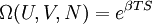
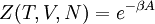
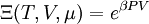
The calculations that can be made over each of these ensembles are explored further in the article Statistical mechanics. The main result for each ensemble however, is its characteristic state function: Microcanonical: Canonical: Grand canonical: For these ensembles, the choice for the appropriate probability measure is dictated by the expressions above. Other thermodynamic ensembles can be also defined, corresponding to different physical requirements, for which analogous formulae can often similarly be derived. Properties of "good" ensemblesThe following properties are considered desirable for a classical mechanical ensemble.
The chosen probability measure on the phase space should be a Gibbs state of the ensemble, i.e. it should be invariant under time evolution. A standard example of this is the natural measure (locally, it is just the Lebesgue measure) on a constant energy surface for a classical mechanical system. Liouville's theorem states this measure is invariant under the Hamiltonian flow.
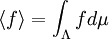
Once a probability measure μ on the phase space Λ is specified, one can define the ensemble average of an observable, i.e. real-valued function f defined on Λ via this measure by
where we have restricted to those observables which are μ-integrable. On the other hand, let provided that this limit exists μ-almost everywhere and is independent of The ergodicity requirement is that the ensemble average coincide with the time average. A sufficient condition for ergodicity is that the time evolution of the system is a mixing. (See also ergodic hypothesis.) Not all systems are ergodic. For instance, it is unknown at this time whether classical mechanical flows on a constant energy surface are ergodic in general. Physically, when a system fails to be ergodic, we may infer that there is more macroscopically discoverable information available about the microscopic state of the system than what we first thought. In turn this may be used to create a better-conditioned ensemble. Ensembles in quantum statistical mechanicsSee main article: Quantum statistical mechanics Putting aside for the moment the question of how statistical ensembles are generated operationally, we should be able to perform the following two operations on ensembles A, B of the same system:
Under certain conditions therefore, equivalence classes of statistical ensembles have the structure of a convex set. In quantum physics, a general model for this convex set is the set of density operators on a Hilbert space. Accordingly, there are two types of ensembles:
Thus a quantum mechanical ensemble is specified by a mixed state in general. For example, one can specify the density operators describing microcanonical, canonical, and grand canonical ensembles of quantum mechanical systems, in a mathematically rigorous fashion. The normalization factor required for the density operator to have trace 1 is the quantum mechanical version of the partition function. We note here that ensembles of quantum mechanical system are sometimes treated by physicists in a semi-classical fashion. Namely, one considers the phase space of the corresponding classical system (e.g. for an ensemble of quantum harmonic oscillators, the phase space of a classical harmonic oscillator is considered). Then, using physical arguments, one derives a suitable "fundamental volume" for the particular system to reflect the fact that quantum mechanical microstates are discretely distributed on the phase space. From the uncertainly principle, it is expected this fundamental volume to be related to the Planck constant, Operational interpretationIn the discussion given so far, while rigorous, we have taken for granted that the notion of an ensemble is valid a priori, as is commonly done in physical context. What has not been shown is that the ensemble itself (not the consequent results) is a precisely defined object mathematically. For instance,
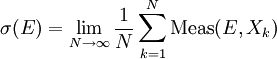
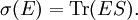
In this section we attempt to partially answer this question. Suppose we have a preparation procedure for a system in a physics lab: For example, the procedure might involve a physical apparatus and some protocols for manipulating the apparatus. As a result of this preparation procedure some system is produced and maintained in isolation for some small period of time. By repeating this laboratory preparation procedure we obtain a sequence of systems X1, X2, ....,Xk, which in our mathematical idealization, we assume is an infinite sequence of systems. The systems are similar in that they were all produced in the same way. This infinite sequence is an ensemble. In a laboratory setting, each one of these prepped systems might be used as input for one subsequent testing procedure. Again, the testing procedure involves a physical apparatus and some protocols; as a result of the testing procedure we obtain a yes or no answer. Given a testing procedure E applied to each prepared system, we obtain a sequence of values Meas (E, X1), Meas (E, X2), ...., Meas (E, Xk). Each one of these values is a 0 (or no) or a 1 (yes). Assume the following time average exists: For quantum mechanical systems, an important assumption made in the quantum logic approach to quantum mechanics is the identification of yes-no questions to the lattice of closed subspaces of a Hilbert space. With some additional technical assumptions one can then infer that states are given by density operators S so that: We see this reflects the definition of quantum states in general: A quantum state is a mapping from the observables to their expectation values. See also |
|
| This article is licensed under the GNU Free Documentation License. It uses material from the Wikipedia article "Statistical_ensemble_(mathematical_physics)". A list of authors is available in Wikipedia. |


 ,
,
 denote a representative point in the phase space, and
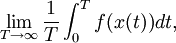
  be its image under the flow, specified by the system in question, at time t. The time average of f is defined to be
 . Accordingly, a ray in a Hilbert space can be used to represent such an ensemble in quantum mechanics. A pure ensemble corresponds to having many copies of the same (up to a global phase) quantum state.
 , in some way.