My watch list

Home
Encyclopedia
Optical_coherence_tomography

Optical coherence tomography

Optical coherence tomography (OCT) is an interferometric, non-invasive optical tomographic imaging technique offering millimeter penetration (approximately 2-3 mm in tissue) with micrometer-scale axial and lateral resolution. The technique was first demonstrated in 1991 with ~30µm axial resolution. Since then, OCT has achieved sub-micrometre resolution in 2001 due to introduction of wide bandwidth light sources (sources emitting wavelengths over a ~100 nm range). By now OCT has found its place as a widely accepted imaging technique, especially in ophthalmology, other biomedical applications and art conservation.

Additional recommended knowledge

What is the Correct Way to Check Repeatability in Balances?

Safe Weighing Range Ensures Accurate Results

Correct Test Weight Handling Guide: 12 Practical Tips

1 Introduction
2 Theory
- 2.1 Time Domain OCT
- 2.2 Frequency Domain OCT (FD-OCT)
  - 2.2.1 Spatially Encoded Frequency Domain OCT (also Fourier Domain OCT)
  - 2.2.2 Time Encoded Frequency Domain OCT (also swept source OCT)
3 Scanning schemes
- 3.1 Single point (confocal) OCT
- 3.2 Parallel OCT
  - 3.2.1 Smart detector array for parallel TD-OCT
4 References
5 See also

Introduction

First devised in 1991 by Huang et al., optical coherence tomography (OCT) with micrometer resolution and cross-sectional imaging capabilities^[1] has become a prominent biomedical tissue-imaging technique; it is particularly suited to ophthalmic applications and other tissue imaging requiring micrometer resolution and millimeter penetration depth^[2]. OCT has also been used for various art conservation projects, where it is used to analyze different layers in a painting. OCT has critical advantages over other medical imaging systems. Medical ultrasonography, magnetic resonance imaging (MRI) and confocal microscopy are not suited to morphological tissue imaging: the first two have poor resolution; the last lacks millimeter penetration depth.^[3]^[4]

OCT is based on low-coherence interferometry.^[5]^[6]^[7] In conventional interferometry with long coherence length (laser interferometry), interference of light occurs over a distance of meters. In OCT, this interference is shortened to a distance of micrometres, thanks to the use of broadband light sources (sources that can emit light over a broad range of frequencies). Light with broad bandwidths can be generated by using superluminescent diodes (superbright LEDs) or lasers with extremely short pulses (femtosecond lasers). White light is also a broadband source with lower powers.

Light in an OCT system is broken into two arms -- a sample arm (containing the item of interest) and a reference arm (usually a mirror). The combination of reflected light from the sample arm and reference light from the reference arm gives rise to an interference pattern, but only if light from both arms have travelled the "same" optical distance ("same" meaning a difference of less than a coherence length). By scanning the mirror in the reference arm, a reflectivity profile of the sample can be obtained (this is time domain OCT). Areas of the sample that reflect back a lot of light will create greater interference than areas that don't. Any light that is outside the short coherence length will not interfere. This reflectivity profile, called an A-scan, contains information about the spatial dimensions and location of structures within the item of interest. A cross-sectional tomograph (B-scan) may be achieved by laterally combining a series of these axial depth scans (A-scan). En face imaging (C-scan) at an acquired depth is possible depending on the imaging engine used.

Theory

The principle OCT is white light or low coherence interferometry. The optical setup typically consists of an interferometer (Fig. 1, typically Michelson type) with a low coherence, broad bandwidth light source. Light is split into and recombined from reference and sample arm, respectively.

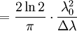
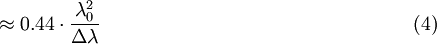
Time Domain OCT

In time domain OCT the pathlength of the reference arm is translated longitudinally in time. A property of low coherence interferometry is that interference, i.e. the series of dark and bright fringes, is only achieved when the path difference lies within the coherence length of the light source. This interference is called auto correlation in a symmetric interferometer (both arms have the same reflectivity), or cross-correlation in the common case. The envelope of this modulation changes as pathlength difference is varied, where the peak of the envelope corresponds to pathlength matching.

The interference of two partially coherent light beams can be expressed in terms of the source intensity, $I S$ , as

$I = k_1 I_S + k_2 I_S + 2 \sqrt { \left ( k_1 I_S \right ) \cdot \left ( k_2 I_S \right )} \cdot Re \left [\gamma \left ( \tau \right ) \right] \qquad (1)$

where $k 1 + k 2 < 1$ represents the interferometer beam splitting ratio, and $γ(τ)$ is called the complex degree of coherence, i.e. the interference envelope and carrier dependent on reference arm scan or time delay $τ$ , and whose recovery of interest in OCT. Due to the coherence gating effect of OCT the complex degree of coherence is represented as a Gaussian function expressed as^[7]

$\gamma \left ( \tau \right ) = \exp \left [- \left ( \frac{\pi\Delta\nu\tau}{2 \sqrt{\ln 2} } \right )^2 \right] \cdot \exp \left ( -j2\pi\nu_0\tau \right ) \qquad \quad (2)$

where $Δν$ represents the spectral width of the source in the optical frequency domain, and $ν 0$ is the centre optical frequency of the source. In equation (2), the Gaussian envelope is amplitude modulated by an optical carrier. The peak of this envelope represents the location of sample under test microstructure, with an amplitude dependent on the reflectivity of the surface. The optical carrier is due to the Doppler effect resulting from scanning one arm of the interferometer, and the frequency of this modulation is controlled by the speed of scanning. Therefore translating one arm of the interferometer has two functions; depth scanning and a Doppler-shifted optical carrier are accomplished by pathlength variation. In OCT, the Doppler-shifted optical carrier has a frequency expressed as

$f_{Dopp} = \frac { 2 \cdot \nu_0 \cdot v_s } { c } \qquad \qquad \qquad \qquad \qquad \qquad \qquad \quad (3)$

where $ν 0$ is the central optical frequency of the source, $v s$ is the scanning velocity of the pathlength variation, and $c$ is the speed of light.

The axial and lateral resolutions of OCT are decoupled from one another; the former being an equivalent to the coherence length of the light source and the latter being a function of the optics. The coherence length of a source and hence the axial resolution of OCT is defined as

$\, {l_c}$	$=\frac {2 \ln 2} {\pi} \cdot \frac {\lambda_0^2} {\Delta\lambda}$
	$\approx 0.44 \cdot \frac {\lambda_0^2} {\Delta\lambda} \qquad \qquad \qquad \qquad \qquad \qquad \qquad \qquad (4)$

Frequency Domain OCT (FD-OCT)

In frequency domain OCT the broadband interference is acquired with spectrally separated detectors (either by encoding the optical frequency in time with a spectrally scanning source or with a dispersive detector, like a grating and a linear detector array). Due to the Fourier relation (Wiener-Khintchine theorem between the auto correlation and the spectral power density) the depth scan can be immediately calculated by a Fourier-transform from the acquired spectra, without movement of the reference arm.^[8] ^[9] This feature improves imaging speed dramatically, while the reduced losses during a single scan improve the signal to noise proportional to the number of detection elements. The parallel detection at multiple wavelength ranges limits the scanning range, while the full spectral bandwidth sets the axial resolution.

Spatially Encoded Frequency Domain OCT (also Fourier Domain OCT)

SEFD-OCT extracts spectral information by distributing different optical frequencies onto a detector stripe (line-array CCD or CMOS) via a dispersive element (see Fig. 1). Thereby the information of the full depth scan can be acquired within a single exposure. However, the large signal to noise advantage of FD-OCT is reduced due the lower dynamic range of stripe detectors in respect to single photosensitive diodes, resulting in an SNR (signal to noise ratio) advantage of ~10 dB at much higher speeds. The drawbacks of this technology are found in a strong fall-off of the SNR, which is proportional to the distance from the zero delay and a sinc-type reduction of the depth dependent sensitivity because of limited detection linewidth. (One pixel detects a quasi-rectangular portion of an optical frequency range instead of a single frequency, the Fourier-transform leads to the sinc(z) behavior). Additionally the dispersive elements in the spectroscopic detector usually do not distribute the light equally spaced in frequency on the detector, but mostly have an inverse dependence. Therefore the signal has to be resampled before processing, which can not take care of the difference in local (pixelwise) bandwidth, which results in further reduction of the signal quality.

Time Encoded Frequency Domain OCT (also swept source OCT)

TEFD-OCT tries to combine some of the advantages of standard TD and SEFD-OCT. Here the spectral components are not encoded by spatial separation, but they are encoded in time. The spectrum either filtered or generated in single successive frequency steps and reconstructed before Fourier-transformation. By accommodation of a frequency scanning light source (i.e. frequency scanning laser) the optical setup (see Fig. 5) becomes simpler than SEFD, but the problem of scanning is essentially translated from the TD-OCT reference-arm into the TEFD-OCT light source. Here the advantage lies in the proven high SNR detection technology, while swept laser sources achieve very small instantaneous bandwidths (=linewidth) at very high frequencies (20-200 kHz). Drawbacks are the nonlinearities in the wavelength, especially at high scanning frequencies. The broadening of the linewidth at high frequencies and a high sensitivity to movements of the scanning geometry or the sample (below the range of nanometers within successive frequency steps)

Scanning schemes

Focusing the light beam to a point on the surface of the sample under test, and recombining the reflected light with the reference will yield an interferogram with sample information corresponding to a single A-scan (Z axis only). Scanning of the sample can be accomplished by either scanning the light on the sample, or by moving the sample under test. A linear scan will yield a two-dimensional data set corresponding to a cross-sectional image (X-Z axes scan), whereas an area scan achieves a three-dimensional data set corresponding to a volumetric image (X-Y-Z axes scan), also called full-field OCT.

Single point (confocal) OCT

Systems based on single point, or flying-spot time domain OCT, must scan the sample in two lateral dimensions and reconstruct a three-dimensional image using depth information obtained by coherence-gating through an axially scanning reference arm (Fig. 2). Two-dimensional lateral scanning has been electromechanically implemented by moving the sample^[9] using a translation stage, and using a novel micro-electro-mechanical system scanner.^[10]

Parallel OCT

Parallel OCT using a charge-coupled device (CCD) camera has been used in which the sample is full-field illuminated and en face imaged with the CCD, hence eliminating the electromechanical lateral scan. By stepping the reference mirror and recording successive en face images a three-dimensional representation can be reconstructed. Three-dimensional OCT using a CCD camera was demonstrated in a phase-stepped technique^[11], using geometric phase-shifting with a Linnik interferometer^[12] , utilising a pair of CCDs and heterodyne detection^[13], and in a Linnik interferometer with an oscillating reference mirror and axial translation stage.^[14] Central to the CCD approach is the necessity for either very fast CCDs or carrier generation separate to the stepping reference mirror to track the high frequency OCT carrier.

Smart detector array for parallel TD-OCT

A two-dimensional smart detector array, fabricated using a 2µm complementary metal-oxide-semiconductor (CMOS) process, was used to demonstrate full-field OCT.^[15] Featuring an uncomplicated optical setup (Fig. 3), each pixel of the 58x58 pixel smart detector array acted as an individual photodiode and included its own hardware demodulation circuitry.

References

^ Huang D, Swanson EA, Lin CP, Schuman JS, Stinson WG, Chang W, Hee MR, Flotte T, Gregory K, Puliafito CA, et al. Optical coherence tomography. Science. 1991 Nov 22;254(5035):1178-81. PMID 1957169.
^ Zysk AM, Nguyen FT, Oldenburg, AL, Marks, DL Boppart SA. Optical coherence tomography: a review of clinical development from bench to bedside. J Biomedical Optics, 12(5):051403, 2007
^ W. Drexler, U. Morgner, R.K. Ghanta, J. S Schuman, F. X Kärtner, J.G. Fujimoto, Nature Medicine, 2001.
^ S. C. Kaufman, D. C. Musch, M. W. Belin, E. J. Cohen, D. M. Meisler, W. J. Reinhart, I. J. Udell and W. S. V. Meter, "Confocal Microscopy: A Report by the American Academy of Ophthalmology", Ophthalmology, vol. 111, no. 2, pp. 396--496, 2004.
^ S. J. Riederer, "Current technical development of magnetic resonance imaging," IEEE Engineering in Medicine and Biology Magazine, vol. 19, no. 5, pp. 34--41, 2000. Available: ieee.org.
^ M. Born and E. Wolf, Principles of Optics: Electromagnetic Theory of Propagation, Interference and Diffraction of Light, Cambridge, Cambridge University Press, 1999.
^ ^a ^b A. F. Fercher, K. Mengedoht, W. Werner, "Eye length measurement by interferometry with partially coherent light," Optics Letters vol. 13, no. 3, pp. 186-188, 1988. Available: opticsinfobase.org.
^ J. M. Schmitt, "Optical Coherence Tomography (OCT): A Review", IEEE Selected Topics in Quantum Electronics, vol. 5, no. 4, pp. 1205--1215, 1999. Available: ieee.org.
^ ^a ^b A. F. Fercher, C. K. Hitzenberger, C. K. Kamp and S. Y. El-Zayat, "Measurement of intraocular distances by backscattering spectral interferometry," Optics Communications vol. 117, no. 1--2, pp. 43--48, (1995. Available: http://dx.doi.org/10.1016/0030-4018(95)00119-S sciencedirect.com].
^ J. T. W. Yeow, V. X. D. Yang, A. Chahwan, M. L. Gordon, B. Qi, I. A. Vitkin, B. C. Wilson and A. A. Goldenberg, "Micromachined 2-D scanner for 3-D optical coherence tomography," Sensors and Actuators A, vol. 117, no. 2, pp. 331-340, 2004. Available: sciencedirect.com.
^ C. Dunsby, Y. Gu and P. M. W. French, "Single-shot phase-stepped wide-field coherence gated imaging," Optics Express, vol. 11, no. 2, pp. 105--115, 2003. Available: opticsinfobase.org.
^ M. Roy, P. Svahn, L. Cherel and C. J. R. Sheppard, "Geometric phase-shifting for low-coherence interference microscopy," Optics and Lasers in Engineering, vol. 37, no. 6, pp. 631--641, 2002. Available: sciencedirect.com.
^ M. Akiba, K. P. Chan and N. Tanno, "Full-field optical coherence tomography by two-dimensional heterodyne detection with a pair of CCD cameras," Optics Letters, vol. 28, no. 10, pp. 816--818, 2003. Available: opticsinfobase.org.
^ A. Dubois, L. Vabre, A.-C. Boccara and E. Beaurepaire, "High-resolution full-field optical coherence tomography with a Linnik microscope," Applied Optics, vol. 41, no. 4, pp. 805--812, 2002. Available: opticsinfobase.org.
^ S. Bourquin, P. Seitz and R. P. Salathé, "Optical coherence tomography based on a two-dimensional smart detector array," Optics Letters, vol. 26, no. 8, pp. 512--514, 2001. Available: opticsinfobase.org.