To use all functions of this page, please activate cookies in your browser.
My watch list
my.chemeurope.com
my.chemeurope.com
With an accout for my.chemeurope.com you can always see everything at a glance – and you can configure your own website and individual newsletter.
- My watch list
- My saved searches
- My saved topics
- My newsletter
Spalart-Allmaras Turbulence ModelSpalart-Allmaras model is a one equation model for the turbulent viscosity. Product highlight
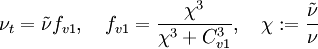
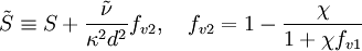
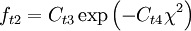
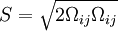
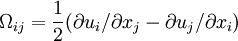
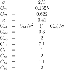
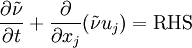
Original modelThe turbulent eddy viscosity is given by The rotation tensor is given by and d is the distance from the closest surface. The constants are Modifications to original modelAccording to Spalart it is safer to use the following values for the last two constants: Other models related to the S-A model: DES (1999) [1] DDES (2006) Model for compressible flowsThere are two approaches to adapting the model for compressible flows. In the first approach the turbulent dynamic viscosity is computed from where ρ is the local density. The convective terms in the equation for where the right hand side (RHS) is the same as in the original model. Boundary conditionsWalls: Freestream: Ideally This is if the trip term is used to "start up" the model. A convenient option is to set Outlet: convective outlet. References
|
|
| This article is licensed under the GNU Free Documentation License. It uses material from the Wikipedia article "Spalart-Allmaras_Turbulence_Model". A list of authors is available in Wikipedia. |


![\frac{\partial \tilde{\nu}}{\partial t} + u_j \frac{\partial \tilde{\nu}}{\partial x_j} = C_{b1} [1 - f_{t2}] \tilde{S} \tilde{\nu} + \frac{1}{\sigma} \{ \nabla \cdot [(\nu + \tilde{\nu}) \nabla \tilde{\nu}] + C_{b2} | \nabla \nu |^2 \} - \left[C_{w1} f_w - \frac{C_{b1}}{\kappa^2} f_{t2}\right] \left( \frac{\tilde{\nu}}{d} \right)^2 + f_{t1} \Delta U^2](images/math/4/7/6/476216889d1ea0604979b921eae3428c.png)
![f_w = g \left[ \frac{ 1 + C_{w3}^6 }{ g^6 + C_{w3}^6 } \right]^{1/6}, \quad g = r + C_{w2}(r^6 - r), \quad r \equiv \frac{\tilde{\nu} }{ \tilde{S} \kappa^2 d^2 }](images/math/0/9/b/09b19885ed6dffe3dec850e2516f1696.png)
![f_{t1} = C_{t1} g_t \exp\left( -C_{t2} \frac{\omega_t^2}{\Delta U^2} [ d^2 + g^2_t d^2_t] \right)](images/math/9/9/3/993b41d0ba795e0b3877d041c4cff1cb.png)


 are modified to

 can be used.
 in the freestream. The model then provides "Fully Turbulent" behavior, i.e., it becomes turbulent in any region that contains shear.


