Dyson series

In scattering theory, the Dyson series is a perturbative series, and each term is represented by Feynman diagrams. This series diverges asymptotically, but in quantum electrodynamics at the second order the difference from experimental data is in the order of 10 ^{− 10}. We get this result because the coupling constant of QED (also known as the fine structure constant) is much less than 1. Notice that in this article ħ = 1.

Additional recommended knowledge

What is the Sensitivity of my Balance?

Don't let static charges disrupt your weighing accuracy

Safe Weighing Range Ensures Accurate Results

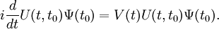
The Dyson operator

We suppose we have a Hamiltonian H which we split into a "free" part H₀ and an "interacting" part V i.e. H=H₀+V. We will work in the interaction picture here.

In the interaction picture, the evolution operator U defined by the equation:

Ψ(t) = U(t,t₀)Ψ(t₀)

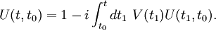
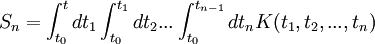
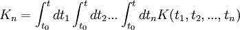
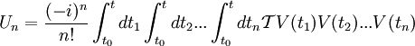
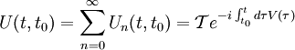
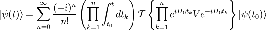
is called Dyson operator.

We have

and then (Tomonaga-Schwinger equation)

Thus:

Derivation of the Dyson series

This leads to the following Neumann series:

If we assume that t > t₁ > t₂ > ... > t_n we can say that the fields are time ordered, and so it is useful to introduce an operator called time-ordering operator. Defining:

We can now try to make this integration simpler. in fact, in the following example:

If K is symmetric in its arguments, we can define (look at integration limits):

And so it is true that:

Returning to our previous integral, it holds the identity:

Summing up all the terms we obtain the Dyson series:

The Dyson series for wavefunctions

Then, going back to the wavefunction for t>t₀,

.

Returning to the Schrödinger picture, for t_f > t_i,

.

References

• Charles J. Joachain, Quantum collision theory, North-Holland Publishing, 1975, ISBN 0-444-86773-2 (Elsevier)