To use all functions of this page, please activate cookies in your browser.
My watch list
my.chemeurope.com
my.chemeurope.com
With an accout for my.chemeurope.com you can always see everything at a glance – and you can configure your own website and individual newsletter.
- My watch list
- My saved searches
- My saved topics
- My newsletter
Atmospheric dispersion modelingAtmospheric dispersion modeling is the mathematical simulation of how air pollutants disperse in the ambient atmosphere. It is performed with computer programs that solve the mathematical equations and algorithms which simulate the pollutant dispersion. The dispersion models are used to estimate or to predict the downwind concentration of air pollutants emitted from sources such as industrial plants and vehicular traffic. Such models are important to governmental agencies tasked with protecting and managing the ambient air quality. The models are typically employed to determine whether existing or proposed new industrial facilities are or will be in compliance with the National Ambient Air Quality Standards (NAAQS) in the United States and other nations. The models also serve to assist in the design of effective control strategies to reduce emissions of harmful air pollutants. The dispersion models require the input of data which includes:
Many of the modern, advanced dispersion modeling programs include a pre-processor module for the input of meteorological and other data, and many also include a post-processor module for graphing the output data and/or plotting the area impacted by the air pollutants on maps. The atmospheric dispersion models are also known as atmospheric diffusion models, air dispersion models, air quality models, and air pollution dispersion models. Product highlight
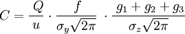
Gaussian air pollutant dispersion equationThe technical literature on air pollution dispersion is quite extensive and dates back to the 1930's and earlier. One of the early air pollutant plume dispersion equations was derived by Bosanquet and Pearson.[1] Their equation did not assume Gaussian distribution nor did it include the effect of ground reflection of the pollutant plume. Sir Graham Sutton derived an air pollutant plume dispersion equation in 1947[2] which did include the assumption of Gaussian distribution for the vertical and crosswind dispersion of the plume and also included the effect of ground reflection of the plume. Under the stimulus provided by the advent of stringent environmental control regulations, there was an immense growth in the use of air pollutant plume dispersion calculations between the late 1960s and today. A great many computer programs for calculating the dispersion of air pollutant emissions were developed during that period of time and they were called "air dispersion models". The basis for most of those models was the Complete Equation For Gaussian Dispersion Modeling Of Continuous, Buoyant Air Pollution Plumes shown below: [3][4]
The above equation not only includes upward reflection from the ground, it also includes downward reflection from the bottom of any inversion lid present in the atmosphere. The sum of the four exponential terms in g3 converges to a final value quite rapidly. For most cases, the summation of the series with m = 1, m = 2 and m = 3 will provide an adequate solution. It should be noted that σz and σy are functions of the atmospheric stability class (i.e., a measure of the turbulence in the ambient atmosphere) and of the downwind distance to the receptor. The two most important variables affecting the degree of pollutant emission dispersion obtained are the height of the emission source point and the degree of atmospheric turbulence. The more turbulence, the better the degree of dispersion. The resulting calculations for air pollutant concentrations are often expressed as an air pollutant concentration contour map in order to show the spatial variation in contaminant levels over a wide area under study. In this way the contour lines can overlay sensitive receptor locations and reveal the spatial relationship of air pollutants to areas of interest. The Briggs plume rise equationsThe Gaussian air pollutant dispersion equation (discussed above) requires the input of H which is the pollutant plume's centerline height above ground level—and H is the sum of Hs (the actual physical height of the pollutant plume's emission source point) plus ΔH (the plume rise due the plume's buoyancy).
To determine ΔH, many if not most of the air dispersion models developed between the late 1960s and the early 2000s used what are known as "the Briggs equations." G.A. Briggs first published his plume rise observations and comparisons in 1965.[5] In 1968, at a symposium sponsored by CONCAWE (a Dutch organization), he compared many of the plume rise models then available in the literature.[6] In that same year, Briggs also wrote the section of the publication edited by Slade[7] dealing with the comparative analyses of plume rise models. That was followed in 1969 by his classical critical review of the entire plume rise literature,[8] in which he proposed a set of plume rise equations which have became widely known as "the Briggs equations". Subsequently, Briggs modified his 1969 plume rise equations in 1971 and in 1972.[9][10] Briggs divided air pollution plumes into these four general categories:
Briggs considered the trajectory of cold jet plumes to be dominated by their initial velocity momentum, and the trajectory of hot, buoyant plumes to be dominated by their buoyant momentum to the extent that their initial velocity momentum was relatively unimportant. Although Briggs proposed plume rise equations for each of the above plume categories, it is important to emphasize that "the Briggs equations" which become widely used are those that he proposed for bent-over, hot buoyant plumes. In general, Briggs's equations for bent-over, hot buoyant plumes are based on observations and data involving plumes from typical combustion sources such as the flue gas stacks from steam-generating boilers burning fossil fuels in large power plants. Therefore the stack exit velocities were probably in the range of 20 to 100 ft/s (6 to 30 m/s) with exit temperatures ranging from 250 to 500 °F (120 to 260 °C). A logic diagram for using the Briggs equations[3] to obtain the plume rise trajectory of bent-over buoyant plumes is presented below:
The above parameters used in the Briggs' equations are discussed in Beychok's book.[3] See alsoAtmospheric dispersion models
Organizations
Others
References
Further readingFor those who would like to learn more about this topic, it is suggested that either one of the following books be read:
Categories: Chemical engineering | Environmental engineering |
|||||||||||||||||||||||||||||||||||||||||||||||||||||||||||||||
| This article is licensed under the GNU Free Documentation License. It uses material from the Wikipedia article "Atmospheric_dispersion_modeling". A list of authors is available in Wikipedia. |


![\exp\;[-\,y^2/\,(2\;\sigma_y^2\;)\;]](images/math/1/d/f/1dff9f22f3889ec5b05d54015f9ab90e.png)

![\; \exp\;[-\,(z - H)^2/\,(2\;\sigma_z^2\;)\;]](images/math/4/0/9/409781e1473eb1aa0b818033f4c2f192.png)
![\;\exp\;[-\,(z + H)^2/\,(2\;\sigma_z^2\;)\;]](images/math/4/3/6/436a30cc4292363ffbbfa0a8e05c38ac.png)
![\sum_{m=1}^\infty\;\big\{\exp\;[-\,(z - H - 2mL)^2/\,(2\;\sigma_z^2\;)\;]](images/math/1/8/c/18cc936e836285e3fbe5e0d3ba17b3bf.png)
![+\, \exp\;[-\,(z + H + 2mL)^2/\,(2\;\sigma_z^2\;)\;]](images/math/3/c/4/3c40697017448bef7cfcfab25939ad4d.png)
![+\, \exp\;[-\,(z + H - 2mL)^2/\,(2\;\sigma_z^2\;)\;]](images/math/8/4/1/8411e4e2a06aae1e25d4d8a89e15e1c3.png)
![+\, \exp\;[-\,(z - H + 2mL)^2/\,(2\;\sigma_z^2\;)\;]](images/math/2/3/c/23c8c3e07bdd7e50ea2f27c52af62f30.png)
Last viewed


