To use all functions of this page, please activate cookies in your browser.
My watch list
my.chemeurope.com
my.chemeurope.com
With an accout for my.chemeurope.com you can always see everything at a glance – and you can configure your own website and individual newsletter.
- My watch list
- My saved searches
- My saved topics
- My newsletter
Electromagnetic reverberation chamber
An electromagnetic reverberation chamber (also known as a reverb chamber (RVC) or mode-stirred chamber (MSC)) is an environment for electromagnetic compatibility (EMC) testing and other electromagnetic investigations. Electromagnetic reverberation chambers have been introduced first by H.A. Mendes in 1968 (Mendes 1968). A reverberation chamber is screened room with a minimum of absorption of electromagnetic energy. Due to the low absorption very high field strength can be achieved with moderate input power. A reverberation chamber is a cavity resonator with a high Q factor. Thus, the spacial distribution of the electrical and magnetical field strength is strongly inhomegenious (standing waves). To reduce this inhomogenity, one or more tuners (stirrers) are used. A tuner is a construction with large metallic reflectors that can be moved to different orientations in order to achieve different boundary conditions. The Lowest Usable Frequency (LUF) of a reverberation chamber depends on the size of the chamber and the design of the tuner. Small chambers have a higher LUF than large chambers. The concept of a reverberation chambers is comparable to a microwave oven. Product highlight
Glossary/NotationPrefaceThe notation is mainly the same as in the IEC standard 61000-4-21(IEC61000-4-21 2003). For statistic quantities like mean and maximal values, a more explicit notation is used in order to emphasize the used domain. Here, spacial domain (subscript s) means that quantities are taken for different chamber positions, and ensemble domain (subscript e) refers to different boundary or excitation conditions (e.g. tuner positions). General
Statistics
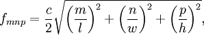
HistoryTheory of OperationCavity ResonatorA reverberation chamber is cavity resonator -- usually a screened room -- that is operated in the overmoded region. To understand what that means we have to investigate cavity resonators briefly. For rectangular cavities, the resonance frequencies (or eigenfrequencies, or natural frequencies) fmnp are given by
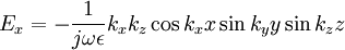
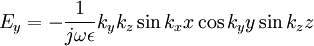
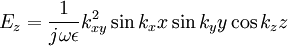
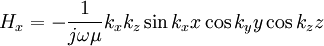
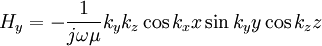
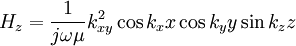
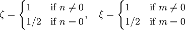
where c is the speed of light, l, w and h are the cavity's length, width and height, and m, n, p are non negative integers (at most one of those can be zero). With that equation, the number of modes with an eigenfrequency less than a given limit f, N(f), can be counted. This results in a stepwise function. In principle, two modes -- a transversal electric mode TEmnp and a transversal magnetic mode TMmnp -- exist for each eigenfrequency. The fields at the chamber position (x,y,z) are given by
 Ex = kycoskxxsinkyysinkzz
 Ey =  − kxsinkxxcoskyysinkzz
Due to the boundary conditions for the E- and H field , some modes does not exist. The restrictions are (Cheng 1989):
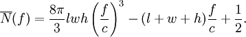
A smooth approximation of N(f),
The leading term is proportional to the chamber volume and to the third power of the frequency. This term is identical to Weyl's formula.
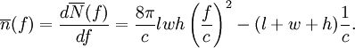
Based on
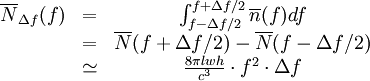
An important quantity is the number of modes in a certain frequency interval Δf,
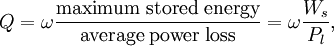
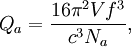
Quality FactorThe Quality Factor (or Q Factor) is an important quatity for all resonant systems. Generally, the Q factor is defined by
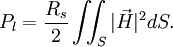
The factor Q of the TE and TM modes can be calculated from the fields. The stored energy Ws is given by
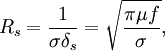
The loss occurs in the metallic walls. If the wall conductivity is σ and the wall permeability is μ, the surface resistance Rs is
where The losses Pl are calculated according to
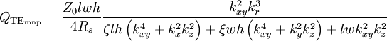
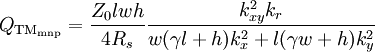
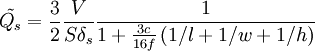
For a rectangular cavity follows (Chang 1989)
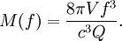
Using the Q values of the individual modes, an averaged Composite Quality Factor
The quality factor including all losses is the harmonic sum of the factors for all single loss processes:
Resulting from the finite quality factor the eigenmodes are broaden in frequency, i.e. a mode can be excited even if the operating frequency does not exactly match the eigenfrequency. Therefore, more eigenmodes are exited for a given frequency at the same time. The Q-bandwidth BWQ is a measure of the frequency bandwidth over which the modes in a reverberation chamber are correlated. The BWQ of a reverberation chamber can be calculated using the following:
Using the formula
Related to the chamber quality factor is the chamber time constant τ by
That is the time constant of the free energy relaxation of the chamber's field (exponential decay) if the input power is switched off. StatisticsAvailable E-FieldTotal Radiated PowerTransientsMeasurementsImmunityEmissionShieldingStandardsIEC 61000-4-21RTCA DO160GMReferences
Electromagnetic Compatibility, 1999 IEEE International Symposium on, Volume 1, 1-6, 2-6 Aug. 1999.
|
|
| This article is licensed under the GNU Free Documentation License. It uses material from the Wikipedia article "Electromagnetic_reverberation_chamber". A list of authors is available in Wikipedia. |


 : Vector of the electric field.
 : Vector of the magnetic field.
 : The total electrical or magnetical field strength, i.e. the magnitude of the field vector.
 : Field strength (magnitude) of one rectangular component of the electrical or magnetical field vector.
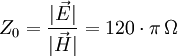 : Characteristic impedance of the free space
 : Power of the forward and backward running waves.
 : spacial mean of
  : ensemble mean of
  : equivalent to
  . Thist is the expected value in statistics.
 : spacial maximum of
  : ensemble maximum of
  : equivalent to
  .
.
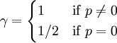
 : max to mean ratio in the spacial domain.
 : max to mean ratio in the ensemble domain.

 , is given by
 is given by
 , that is given by
 where the maximum and the average are taken over one cycle, and
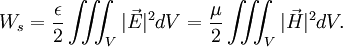
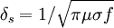 is the skin depth of the wall material.
 can be derived
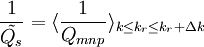
 where
where