To use all functions of this page, please activate cookies in your browser.
My watch list
my.chemeurope.com
my.chemeurope.com
With an accout for my.chemeurope.com you can always see everything at a glance – and you can configure your own website and individual newsletter.
- My watch list
- My saved searches
- My saved topics
- My newsletter
Gibbs samplingIn mathematics and physics, Gibbs sampling is an algorithm to generate a sequence of samples from the joint probability distribution of two or more random variables. The purpose of such a sequence is to approximate the joint distribution (i.e. to generate a histogram), or to compute an integral (such as an expected value). Gibbs sampling is a special case of the Metropolis-Hastings algorithm, and thus an example of a Markov chain Monte Carlo algorithm. The algorithm is named after the physicist J. W. Gibbs, in reference to an analogy between the sampling algorithm and statistical physics. The algorithm was devised by Geman and Geman (citation below), some eight decades after the passing of Gibbs, and is also called the Gibbs sampler. Gibbs sampling is applicable when the joint distribution is not known explicitly, but the conditional distribution of each variable is known. The Gibbs sampling algorithm is to generate an instance from the distribution of each variable in turn, conditional on the current values of the other variables. It can be shown (see, for example, Gelman et al.) that the sequence of samples comprises a Markov chain, and the stationary distribution of that Markov chain is just the sought-after joint distribution. Gibbs sampling is particularly well-adapted to sampling the posterior distribution of a Bayesian network, since Bayesian networks are typically specified as a collection of conditional distributions. BUGS (link below) is a program for carrying out Gibbs sampling on Bayesian networks. Product highlight
BackgroundGibbs sampling is a special case of Metropolis-Hastings sampling but the value is always accepted ( ImplementationSuppose that a sample
These steps define a reversible markov chain with the desired invariant distribution and so the detailed balance equations are satisfied showing that the chain is reversible, and that it has invariant distribution In practice, the suffix Failure ModesThere are two ways that Gibbs sampling can fail. The first is when there are islands of high-probability states, with no paths between them. For example, consider a probability distribution over 2-bit vectors, where the vectors (0,0) and (1,1) each have probability 1/2, but the other two vectors (0,1) and (1,0) have probability zero. Gibbs sampling will become trapped in one of the two high-probability vectors, and will never reach the other one. More generally, for any distribution over high-dimensional, real-valued vectors, if 2 particular elements of the vector are perfectly correlated (or perfectly anti-correleated), those 2 elements will become stuck, and Gibbs sampling will never be able to change them. The second problem can happen even when all states have nonzero probability and there is only a single island of high-probability states. For example, consider a probability distribution over 100-bit vectors, where the all-zeros vector occurs with probability 1/2, and all other vectors are equally probable, and so have a probability of This problem occurs no matter how long the burn in period is. This is because in the true distribution, the zero vector occurs half the time, and those occurances are randomly mixed in with the nonzero vectors. Even a small sample will see both zero and nonzero vectors. But Gibbs sampling will alternate between returning only the zero vector for long periods (about 299 in a row), then only nonzero vectors for long periods (about 299 in a row). So in the long term it has the correct distribution of giving the zero vector with probability 1/2. But for a typical sample size that can be obtained in less than a century, the zero vector will either appear with probability 0 or probability 1 in the sample. So in this case, Gibbs sampling works in theory but fails in practice. See also
References
|
|
| This article is licensed under the GNU Free Documentation License. It uses material from the Wikipedia article "Gibbs_sampling". A list of authors is available in Wikipedia. |


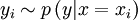
 ). The point of Gibbs sampling is that given a multivariate distribution it is simpler to sample from a conditional distribution rather than integrating over a joint distribution. Suppose we want to sample
  values of
  from a joint distribution
  . We begin with a value of
  and sample
  . Once that value of
  :
:  .
.
 is taken from a distribution depending on a parameter vector
  of length
  , with prior distribution
  . It may be that
  would be computationally expensive. Then an alternative method of calculating the marginal densities is to create a Markov chain on the space
  by repeating these two steps:

 according to
 . This
can be proven as follows. Define
. This
can be proven as follows. Define  for all
  and let
  denote the probability of a jump from
  to
to  . Then, for
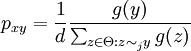
 otherwise. So
 is not chosen at random, and the chain cycles through the suffixes in order. In general this gives a non-reversible chain, but it will still have the desired invariant distribution (as long as the chain can access all states under the fixed ordering).
 each. If you want to know the probability of the zero vector, it would be sufficient to take 100 or 1000 samples from the true distribution. That would very likely give an answer very close to 1/2. But you would probably have to take more than
 Last viewed


