To use all functions of this page, please activate cookies in your browser.
My watch list
my.chemeurope.com
my.chemeurope.com
With an accout for my.chemeurope.com you can always see everything at a glance – and you can configure your own website and individual newsletter.
- My watch list
- My saved searches
- My saved topics
- My newsletter
Metropolis-Hastings algorithm
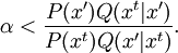
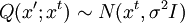
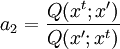
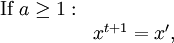
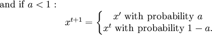
Product highlightIn mathematics and physics, the Metropolis-Hastings algorithm is a rejection sampling algorithm used to generate a sequence of samples from a probability distribution that is difficult to sample from directly. This sequence can be used in Markov chain Monte Carlo simulation to approximate the distribution (i.e., to generate a histogram), or to compute an integral (such as an expected value). The algorithm was named in reference to Nicholas Metropolis, who published it in 1953 for the specific case of the Boltzmann distribution, and W.K. Hastings,[1] who generalized it in 1970. The Gibbs sampling algorithm is a special case of the Metropolis-Hastings algorithm which is usually faster and easier to use but is less generally applicable. The Metropolis-Hastings algorithm can draw samples from any probability distribution P(x), requiring only that a function proportional to the density can be calculated at x. In Bayesian applications, the normalization factor is often extremely difficult to compute, so the ability to generate a sample without knowing this constant of proportionality is a major virtue of the algorithm. The algorithm generates a Markov chain in which each state xt + 1 depends only on the previous state xt. The algorithm uses a proposal density Q(x';xt), which depends on the current state xt, to generate a new proposed sample x'. This proposal is 'accepted' as the next value (xt + 1=x') if α drawn from U(0,1) is If the proposal is not accepted, then the current value of x is retained: xt + 1 = xt. For example, the proposal density could be a Gaussian function centred on the current state xt: reading Q(x';xt) as the probability density function for x' given the previous value xt. This proposal density would generate samples centred around the current state with variance σ2I. The original Metropolis algorithm calls for the proposal density to be symmetric ( Q(x;y) = Q(y;x) ); the generalization by Hastings lifts this restriction. It is also permissible for Q(x',xt) not to depend on x' at all, in which case the algorithm is called "Independence Chain Metropolis-Hastings" ( as opposed to "Random Walk Metropolis-Hastings" ). The Independence Chain M-H algorithm with a suitable proposal density function can offer higher accuracy than the random walk version, but it requires some a priori knowledge of the distribution. Step-by-step instructionsSuppose the most recent value sampled is xt. To follow the Metropolis-Hastings algorithm, we next draw a new proposal state x' with probability Q(x';xt), and calculate a value where is the likelihood ratio between the proposed sample x' and the previous sample xt, and is the ratio of the proposal density in two directions (from xt to x' and vice versa). This is equal to 1 if the proposal density is symmetric. Then the new state xt + 1 is chosen according to the following rules. The Markov chain is started from a random initial value x0 and the algorithm is run for many iterations until this initial state is "forgotten". These samples, which are discarded, are known as burn-in. The remaining set of accepted values of x represent a sample from the distribution P(x).
The algorithm works best if the proposal density matches the shape of the target distribution P(x), that is See also
References
|
| This article is licensed under the GNU Free Documentation License. It uses material from the Wikipedia article "Metropolis-Hastings_algorithm". A list of authors is available in Wikipedia. |


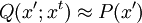 , but in most cases this is unknown.
If a Gaussian proposal density
, but in most cases this is unknown.
If a Gaussian proposal density Last viewed


