My watch list

Kuramoto model

The Kuramoto model, first proposed by Yoshiki Kuramoto (蔵本由紀 Kuramoto Yoshiki), is a mathematical model used to describe synchronization. More specifically, it is a model for the behavior of a large set of coupled oscillators. Its formulation was motivated by the behavior of systems of chemical and biological oscillators, and it has found widespread applications.

The model makes several assumptions, including that there is weak coupling, identical or nearly identical oscillators, and that interactions that depend sinusoidally on the phase difference between the two objects.

Additional recommended knowledge

How to ensure accurate weighing results every day?

Recognize and detect the effects of electrostatic charges on your balance

Guide to balance cleaning: 8 simple steps

1 Definition
2 Transformation
3 Large N limit
4 Solutions
5 References

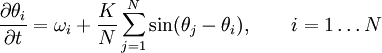
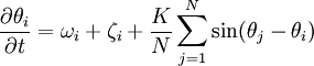
Definition

In the most popular version of the Kuramoto model, each of the oscillators is considered to have its own intrinsic natural frequency $ω i$ , and each is coupled equally to all other oscillators. Surprisingly, this fully nonlinear model can be solved exactly, in the infinite-N limit, with a clever transformation and the application of self-consistency arguments.

The most popular form of the model has the following governing equations:

$\frac{\partial \theta_i}{\partial t} = \omega_i + \frac{K}{N} \sum_{j=1}^{N} \sin(\theta_j - \theta_i), \qquad i = 1 \ldots N$ ,

where the system is composed of N limit-cycle oscillators.

Noise can be added to the system. In that case, the original equation is altered to:

$\frac{\partial \theta_i}{\partial t} = \omega_{i}+\zeta_{i}+\dfrac{K}{N}\sum_{j=1}^N\sin(\theta_{j}-\theta_{i})$ ,

where $ζ i$ is the fluctuation and a function of time. If we consider the noise to be white noise, then

$\langle\zeta_{i}(t)\rangle=0$ ,

$\langle\zeta_{i}(t)\zeta_{j}(t')\rangle=2D\delta_{ij}\delta(t-t')$

with $D$ denotes the strength of noise.

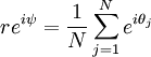
Transformation

The transformation that allows this model to be solved exactly (at least in the N → ∞ limit) is as follows. Define the "order" parameters r and ψ as

$re^{i \psi} = \frac{1}{N} \sum_{j=1}^{N} e^{i \theta_j}$ .

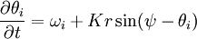
Here r represents the phase-coherence of the population of oscillators, and ψ indicates the average phase. Applying this transformation, the governing equation becomes

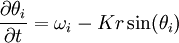
$\frac{\partial \theta_i}{\partial t} = \omega_i + K r \sin(\psi-\theta_i)$ .

Thus the oscillators' equations are no longer explicitly coupled; instead the order parameters govern behavior. A further transformation is usually done, to a rotating frame in which the statistical average of phases over all oscillators is zero. That is, $ψ = 0$ . Finally, the governing equation becomes

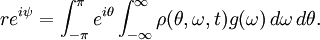
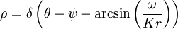
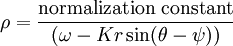
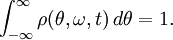
$\frac{\partial \theta_i}{\partial t} = \omega_i - K r \sin(\theta_i)$ .

Large N limit

Now consider the case as N tends to infinity. Take the distribution of intrinsic natural frequencies as g(ω) (assumed normalized). Then assume that the density of oscillators at a given phase θ, with given natural frequency ω, at time t is $ρ(θ,ω, t)$ . Normalization requires that

$\int_{-\infty}^{\infty} \rho(\theta, \omega, t) \, d \theta = 1.$

The continuity equation for oscillator density will be

$\frac{\partial \rho}{\partial t} + \frac{\partial}{\partial \theta}[\rho v] = 0,$

where v is the drift velocity of the oscillators given by taking the infinite-N limit in the transformed governing equation, i.e.,

$\frac{\partial \rho}{\partial t} + \frac{\partial}{\partial \theta}[\rho \omega + \rho K r \sin(\psi-\theta)] = 0.$

Finally, we must rewrite the definition of the order parameters for the continuum (infinite N) limit. $θ i$ must be replaced by its ensemble average (over all ω) and the sum must be replaced by an integral, to give

$r e^{i \psi} = \int_{-\pi}^{\pi} e^{i \theta} \int_{-\infty}^{\infty} \rho(\theta, \omega, t) g(\omega) \, d \omega \, d \theta.$

Solutions

The incoherent state with all oscillators drifting randomly corresponds to the solution $ρ = 1 / (2π)$ . In that case $r = 0$ , and there is no coherence among the oscillators. They are uniformly distributed across all possible phases, and the population is in a statistical steady-state (although individual oscillators continue to change phase in accordance with their intrinsic ω).

When coupling K is sufficiently strong, a fully synchronized solution is possible. In the fully synchronized state, all the oscillators share a common frequency, although their phases are different.

A solution for the case of partial synchronization yields a state in which only some oscillators (those near the ensemble's mean natural frequency) synchronize; other oscillators drift incoherently. Mathematically, the state has

$\rho = \delta\left(\theta - \psi - \arcsin\left(\frac{\omega}{K r}\right)\right)$

for locked oscillators, and

$\rho = \frac{\rm{normalization \; constant}}{(\omega - K r \sin(\theta - \psi))}$

for drifting oscillators. The cutoff occurs when $| ω | < K r$ .

References

Acebrón, Juan A.; Bonilla, L. L.; Pérez Vicente, Conrad J.; Ritort, Félix; Spigler, Renato. The Kuramoto model: a simple paradigm for synchronization phenomena [1]

Strogatz, S. From Kuramoto to Crawford: exploring the onset of synchronization in populations of coupled oscillators, Physica D 143 (2000) 1–20

Category: Lattice models

This article is licensed under the GNU Free Documentation License. It uses material from the Wikipedia article "Kuramoto_model". A list of authors is available in Wikipedia.