My watch list

Home
Encyclopedia
Lippmann-Schwinger_equation

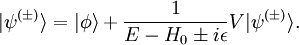
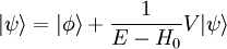
Lippmann-Schwinger equation

The Lippmann-Schwinger equation (named after Bernard A. Lippmann and Julian Schwinger) is of importance to scattering theory. The equation is

$| \psi^{(\pm)} \rangle = | \phi \rangle + \frac{1}{E - H_0 \pm i \epsilon} V |\psi^{(\pm)} \rangle. \,$

Additional recommended knowledge

What is the Correct Way to Check Repeatability in Balances?

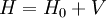
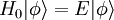
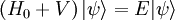
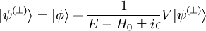
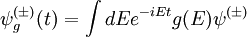
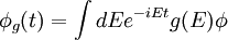
Derivation

We will assume that the Hamiltonian may be written as

$H = H_0 + V \,$

where H and H₀ have the same eigenvalues and H₀ is a free Hamiltonian. For example in nonrelativistic quantum mechanics H₀ may be

$H_0 = \frac{p^2}{2m}. \,$

Intuitively $V \,$ is the interaction energy of the system. This analogy is somewhat misleading, as interactions generically change the energy levels E of steady states of the system, but H and H₀ have identical spectra E_α. This means that, for example, a bound state that is an eigenstate of the interacting Hamiltonian will also be an eigenstate of the free Hamiltonian. This is in contrast with the Hamiltonian obtained by turning off all interactions, in which case there would be no bound states. Thus one may think of H₀ as the free Hamiltonian for the boundstates with effective parameters that are determined by the interactions.

Let there be an eigenstate of $H_0 \,$ :

$H_0 | \phi \rangle = E | \phi \rangle \,$

Now if we add the interaction $V \,$ into the mix, we need to solve

$\left( H_0 + V \right) | \psi \rangle = E | \psi \rangle \,$

Because of the continuity of the energy eigenvalues, we wish that $| \psi \rangle \to | \phi \rangle \,$ as $V \to 0 \,$ .

A potential solution to this situation is

$|\psi \rangle = | \phi \rangle + \frac{1}{E - H_0} V | \psi \rangle \,$

However $(E - H 0)$ is singular since $E$ is an eigenvalue of $H 0$ .

As is described below, this singularity is eliminated in two distinct ways by making the denominator slightly complex:

$| \psi^{(\pm)} \rangle = | \phi \rangle + \frac{1}{E - H_0 \pm i \epsilon} V |\psi^{(\pm)} \rangle \,$

Interpretation as in and out states

The S-matrix paradigm

In the S-matrix formulation of quantum field theory, which was pioneered by John Archibald Wheeler among others, all physical processes are modeled according to the following paradigm.

One begins with a non-interacting multiparticle state in the distant past. Non-interacting does not mean that all of the forces have been turned off, in which case for example protons would fall apart, but rather that there exists an interaction-free Hamiltonian H₀ for the bound states which has the same spectrum as the actual Hamiltonian H. This initial state is referred to as the in state. Intuitively it consists of boundstates that are sufficiently well separated that their interactions with each other are ignored.

The idea is that whatever physical process one is trying to study may be modeled as a scattering process of these well separated bound states. This process is described by the full Hamiltonian H, but once its over all of the new bound states separate again and one finds a new noninteracting state called the out state.

This paradigm allows one to calculate the probabilities of all of the processes that we have observed in 70 years of particle collider experiments with remarkable accuracy. That said, many interesting physical phenomena do not fit into the above paradigm. For example, if one wishes to consider the dynamics inside of a neutron star sometimes one wants to know more than what it will finally decay into. In other words, one may be interested in measurements that are not in the asymptotic future. Sometimes an asymptotic past or future is not even available. For example, it is very possible that there is no past before the big bang, and in general relativity the future of system falling into a Schwarzschild black hole ends at a singularity and not in a well-separated asymptotic future.

The connection to Lippmann-Schwinger

Intuitively, the slightly deformed eigenfunctions $\psi^{(\pm)}$ of the full Hamiltonian H are the in and out states. The $φ$ are noninteracting states that resemble the in and out states in the infinite past and infinite future.

Creating wavepackets

This intuitive picture is not quite right, because $\psi^{(\pm)}$ is an eigenfunction of the Hamiltonian and so at different times only differs by a phase, and so in particular the physical state does not evolve and so it cannot become noninteracting. This problem is easily circumvented by assembling $\psi^{(\pm)}$ and $φ$ into wavepackets with some distribution g(E) of energies E over a characteristic scale $Δ E$ . The uncertainty principle now allows the interactions of the asymptotic states to occur over a timescale $\hbar/\Delta E$ and in particular it is no longer inconceivable that the interactions may turn off outside of this interval. The following argument suggests that this is indeed the case.

Plugging the Lippmann-Schwinger equations into the definitions

$\psi^{(\pm)}_g(t)=\int dE e^{-iEt} g(E)\psi^{(\pm)}$

and

$\phi_g(t)=\int dE e^{-iEt} g(E)\phi$

of the wavepackets we see that, at a given time, the difference between the $ψ g (t)$ and $φ g (t)$ wavepackets is given by an integral over the energy E.

A contour integral

This integral may be evaluated by defining the wave function over the complex E plane and closing the E contour using a semicircle on which the wavefunctions vanish. The integral over the closed contour may then be evaluated, using the Cauchy integral theorem, as a sum of the residues at the various poles. We will now argue that the residues of $\psi^{(\pm)}$ approach those of $φ$ at time $t\rightarrow\mp\infty$ and so the corresponding wavepackets are equal at temporal infinity.

In fact, for very positive times t the $e - i E t$ factor in a Schrödinger picture state forces one to close the contour on the lower half-plane. The pole in the V from the Lippmann-Schwinger equation reflects the time-uncertainty of the interaction, while that in the wavepackets weight function reflects the duration of the interaction. Both of these varieties of poles occur at finite imaginary energies and so are suppressed at very large times. The pole in the energy difference in the denominator is on the upper half-plane in the case of $ψ -$ , and so does not lie inside the integral contour and does not contribute to the $ψ -$ integral. The remainder is equal to the $φ$ wavepacket. Thus, at very late times $ψ - = φ$ , identifying $ψ -$ as the asymptotic noninteracting out state.

Similarly one may integrate the wavepacket corresponding to $ψ +$ at very negative times. In this case the contour needs to be closed over the upper half-plane, which therefore misses the energy pole of $ψ +$ , which is in the lower half-plane. One then finds that the $ψ +$ and $φ$ wavepackets are equal in the asymptotic past, identifying $ψ +$ as the asymptotic noninteracting in state.

The complex denominator of Lippmann-Schwinger

This identification of the $ψ$ 's as asymptotic states is the justification for the $\pm\epsilon$ in the denominator of the Lippmann-Schwinger equations.

A formula for the S-matrix

The S-matrix S is defined to be the inner product

$S_{ab}=(\psi^-_a,\psi^+_b)$

of the ath and bth Heisenberg picture asymptotic states. One may obtain a formula relating the S-matrix to the potential V using the above contour integral strategy, but this time switching the roles of $ψ +$ and $ψ -$ . As a result, the countour now does pick up the energy pole. This can be related to the $φ$ 's if one uses the S-matrix to swap the two $ψ$ 's. Identifying the coefficients of the $φ$ 's on both sides of the equation one finds the desired formula relating S to the potential

$S_{ab}=\delta(a-b)-2i\pi\delta(E_a-E_b)(\phi_b,V\psi^+_a).$

In the Born approximation, corresponding to first order perturbation theory, one replaces this last $ψ +$ with the corresponding eigenfunction $φ$ of the free Hamiltonian H₀, yielding

$S_{ab}=\delta(a-b)-2i\pi\delta(E_a-E_b)(\phi_b,V\phi_a)\,$

which expresses the S-matrix entirely in terms of V and free Hamiltonian eigenfunctions.

These formulas may in turn be used to calculate the reaction rate of the process $b\rightarrow a$ , which is equal to $|S_{ab}-\delta_{ab}|^2.\,$

References

Sakurai, J. J. (1994). Modern Quantum Mechanics. Addison Wesley. ISBN 0-201-53929-2.

Weinberg, S. (1995). The Quantum Theory of Fields. Cambridge University Press. ISBN 0-521-67053-5.

Category: Scattering

This article is licensed under the GNU Free Documentation License. It uses material from the Wikipedia article "Lippmann-Schwinger_equation". A list of authors is available in Wikipedia.