To use all functions of this page, please activate cookies in your browser.
My watch list
my.chemeurope.com
my.chemeurope.com
With an accout for my.chemeurope.com you can always see everything at a glance – and you can configure your own website and individual newsletter.
- My watch list
- My saved searches
- My saved topics
- My newsletter
Monte Carlo integrationIn mathematics, Monte Carlo integration is numerical quadrature using pseudorandom numbers. That is, Monte Carlo integration methods are algorithms for the approximate evaluation of definite integrals, usually multidimensional ones. The usual algorithms evaluate the integrand at a regular grid. Monte Carlo methods, however, randomly choose the points at which the integrand is evaluated. Informally, to estimate the area of a domain D, first pick a simple domain d whose area is easily calculated and which contains D. Now pick a sequence of random points that fall within d. Some fraction of these points will also fall within D. The area of D is then estimated as this fraction multiplied by the area of d. The traditional Monte Carlo algorithm distributes the evaluation points uniformly over the integration region. Adaptive algorithms such as VEGAS and MISER use importance sampling and stratified sampling techniques to get a better result. Product highlight
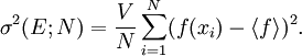
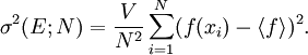
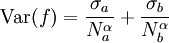
The traditional algorithmThe algorithm computes an estimate of a multidimensional definite integral of the form, over the hypercube with volume V defined by { (x, y, …) | xl ≤ x ≤ xu, yl ≤ y ≤ yu, … }. The plain Monte Carlo algorithm samples points uniformly from the integration region to estimate the integral and its error. Suppose that the sample has size N and denote the points in the sample by x1, …, xN. Then the estimate for the integral is given by where The variance of the function can be estimated using The variance of the estimate of the integral can be estimated using For large N this variance decreases asymptotically as var(f) / N, where var(f) is the true variance of the function over the integration region. The error estimate itself should decrease as σ(f) / √N. The familiar law of errors decreasing as 1 / √N applies: to reduce the error by a factor of 10 requires a 100-fold increase in the number of sample points. The above expression provides a statistical estimate of the error on the result. This error estimate is not a strict error bound — random sampling of the region may not uncover all the important features of the function, resulting in an underestimate of the error. MISER Monte CarloThe MISER algorithm of Press and Farrar is based on recursive stratified sampling. This technique aims to reduce the overall integration error by concentrating integration points in the regions of highest variance. The idea of stratified sampling begins with the observation that for two disjoint regions a and b with Monte Carlo estimates of the integral Ea(f) and Eb(f) and variances It can be shown that this variance is minimized by distributing the points such that,
Hence the smallest error estimate is obtained by allocating sample points in proportion to the standard deviation of the function in each sub-region. The MISER algorithm proceeds by bisecting the integration region along one coordinate axis to give two sub-regions at each step. The direction is chosen by examining all d possible bisections and selecting the one which will minimize the combined variance of the two sub-regions. The variance in the sub-regions is estimated by sampling with a fraction of the total number of points available to the current step. The same procedure is then repeated recursively for each of the two half-spaces from the best bisection. The remaining sample points are allocated to the sub-regions using the formula for N_a and N_b. This recursive allocation of integration points continues down to a user-specified depth where each sub-region is integrated using a plain Monte Carlo estimate. These individual values and their error estimates are then combined upwards to give an overall result and an estimate of its error. This routines uses the MISER Monte Carlo algorithm to integrate the function f over the dim-dimensional hypercubic region defined by the lower and upper limits in the arrays xl and xu, each of size dim. The integration uses a fixed number of function calls, and obtains random sampling points using the random number generator r. A previously allocated workspace s must be supplied. The result of the integration is returned in result, with an estimated absolute error abserr. Configurable ParametersThe MISER algorithm has several configurable parameters. estimate_fracThis parameter specifies the fraction of the currently available number of function calls which are allocated to estimating the variance at each recursive step. In the GNU Scientific Library's implementation, the default value is 0.1. min_callsThis parameter specifies the minimum number of function calls required for each estimate of the variance. If the number of function calls allocated to the estimate using estimate_frac falls below min_calls then min_calls are used instead. This ensures that each estimate maintains a reasonable level of accuracy. In the GNU Scientific Library's implementation, the default value of min_calls is 16 * dim. min_calls_per_bisectionThis parameter specifies the minimum number of function calls required to proceed with a bisection step. When a recursive step has fewer calls available than min_calls_per_bisection it performs a plain Monte Carlo estimate of the current sub-region and terminates its branch of the recursion. In the GNU Scientific Library's implementation, the default value of this parameter is 32 * min_calls. alphaThis parameter controls how the estimated variances for the two sub-regions of a bisection are combined when allocating points. With recursive sampling the overall variance should scale better than 1/N, since the values from the sub-regions will be obtained using a procedure which explicitly minimizes their variance. To accommodate this behavior the MISER algorithm allows the total variance to depend on a scaling parameter \alpha, The authors of the original paper describing MISER recommend the value α = 2 as a good choice, obtained from numerical experiments, and this is used as the default value in the GNU Scientific Library's implementation. ditherThis parameter introduces a random fractional variation of size dither into each bisection, which can be used to break the symmetry of integrands which are concentrated near the exact center of the hypercubic integration region. In the GNU Scientific Library's implementation, the default value of dither is zero, so no variation is introduced. If needed, a typical value of dither is around 0.1. VEGAS Monte CarloThe VEGAS algorithm of G.P.Lepage is based on importance sampling. It samples points from the probability distribution described by the function | f | , so that the points are concentrated in the regions that make the largest contribution to the integral. In general, if the Monte Carlo integral of f is sampled with points distributed according to a probability distribution described by the function g, we obtain an estimate Eg(f;N), Eg(f;N) = E(f / g;N) with a corresponding variance, Varg(f;N) = Var(f / g;N) If the probability distribution is chosen as g = | f | / I( | f | ) then it can be shown that the variance Vg(f;N) vanishes, and the error in the estimate will be zero. In practice it is not possible to sample from the exact distribution g for an arbitrary function, so importance sampling algorithms aim to produce efficient approximations to the desired distribution. The VEGAS algorithm approximates the exact distribution by making a number of passes over the integration region while histogramming the function f. Each histogram is used to define a sampling distribution for the next pass. Asymptotically this procedure converges to the desired distribution. In order to avoid the number of histogram bins growing like Kd the probability distribution is approximated by a separable function: VEGAS incorporates a number of additional features, and combines both stratified sampling and importance sampling. The integration region is divided into a number of "boxes", with each box getting a fixed number of points (the goal is 2). Each box can then have a fractional number of bins, but if bins/box is less than two, Vegas switches to a kind variance reduction (rather than importance sampling). This routines uses the VEGAS Monte Carlo algorithm to integrate the function f over the dim-dimensional hypercubic region defined by the lower and upper limits in the arrays xl and xu, each of size dim. The integration uses a fixed number of function calls calls, and obtains random sampling points using the random number generator r. A previously allocated workspace s must be supplied. The result of the integration is returned in result, with an estimated absolute error abserr. The result and its error estimate are based on a weighted average of independent samples. The chi-squared per degree of freedom for the weighted average is returned via the state struct component, The VEGAS algorithm computes a number of independent estimates of the integral internally, according to the iterations parameter described below, and returns their weighted average. Random sampling of the integrand can occasionally produce an estimate where the error is zero, particularly if the function is constant in some regions. An estimate with zero error causes the weighted average to break down and must be handled separately. In the original Fortran implementations of VEGAS the error estimate is made non-zero by substituting a small value (typically 1e-30). The implementation in GSL differs from this and avoids the use of an arbitrary constant -- it either assigns the value a weight which is the average weight of the preceding estimates, or discards it according to the following procedure:
Configurable ParametersThe VEGAS algorithm is configurable. chisqThis parameter gives the chi-squared per degree of freedom for the weighted estimate of the integral. The value of chisq should be close to 1. A value of chisq which differs significantly from 1 indicates that the values from different iterations are inconsistent. In this case the weighted error will be under-estimated, and further iterations of the algorithm are needed to obtain reliable results. alphaThe parameter alpha controls the stiffness of the rebinning algorithm. It is typically set between one and two. A value of zero prevents rebinning of the grid. In the GNU Scientific Library's implementation, the default value is 1.5. iterationsThe number of iterations to perform for each call to the routine. In the GNU Scientific Library's implementation, the default value is 5 iterations. stageSetting this determines the stage of the calculation. Normally, stage = 0 which begins with a new uniform grid and empty weighted average. Calling vegas with stage = 1 retains the grid from the previous run but discards the weighted average, so that one can "tune" the grid using a relatively small number of points and then do a large run with stage = 1 on the optimized grid. Setting stage = 2 keeps the grid and the weighted average from the previous run, but may increase (or decrease) the number of histogram bins in the grid depending on the number of calls available. Choosing stage = 3 enters at the main loop, so that nothing is changed, and is equivalent to performing additional iterations in a previous call. modeThe possible choices are GSL_VEGAS_MODE_IMPORTANCE, GSL_VEGAS_MODE_STRATIFIED, GSL_VEGAS_MODE_IMPORTANCE_ONLY. This determines whether VEGAS will use importance sampling or stratified sampling, or whether it can pick on its own. In low dimensions VEGAS uses strict stratified sampling (more precisely, stratified sampling is chosen if there are fewer than 2 bins per box). References and further readingThe MISER algorithm is described in the following article,
The VEGAS algorithm is described in the following papers,
Based on the GNU Scientific Library's manual, which is published under the GFDL (and hence free to use for Wikipedia). Original available here. |
|
| This article is licensed under the GNU Free Documentation License. It uses material from the Wikipedia article "Monte_Carlo_integration". A list of authors is available in Wikipedia. |


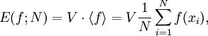
 denotes the sample mean of the integrand.
 and
and  , the variance
 so that the number of bins required is only
  , and must be consistent with 1 for the weighted average to be reliable.
Last viewed


