To use all functions of this page, please activate cookies in your browser.
My watch list
my.chemeurope.com
my.chemeurope.com
With an accout for my.chemeurope.com you can always see everything at a glance – and you can configure your own website and individual newsletter.
- My watch list
- My saved searches
- My saved topics
- My newsletter
Monte Carlo methods in financeIn the fields of finance and mathematical finance, Monte Carlo methods are used to value and analyze basic financial models through to complex instruments, portfolios and investments by simulating the various sources of uncertainty affecting their value, and then determining their average value over the range of resultant outcomes [1]. The advantage of Monte Carlo methods over other techniques increases as the dimensions (sources of uncertainty) of the problem increase. Monte Carlo methods were first introduced to finance in 1977 by Phelim Boyle in his seminal paper "Options: A Monte Carlo Approach" in the Journal of Financial Economics. This article discusses typical financial problems in which Monte Carlo methods are used. It also touches on the use of so-called "quasi-random" methods such as the use of Sobol sequences. Product highlight
OverviewThe Monte Carlo Method encompasses any technique of statistical sampling employed to approximate solutions to quantitative problems [2]. Essentially, the Monte Carlo method solves a problem by directly simulating the underlying physical process and then calculating the (average) result of the process [3]. This very general approach is valid in areas such as physics, chemistry, computer science etc. In finance, the Monte Carlo method is used to simulate the various sources of uncertainty that affect the value of the instrument, portfolio or investment in question, and to then calculate a representative value given these possible values of the underlying inputs [4]. This approach is therefore used by financial analysts who wish to construct "stochastic" or probabilistic financial models as opposed to the traditional static and deterministic models. Some examples:
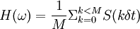
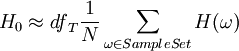
Note that, in general, simulation methods are preferred to other valuation techniques only when there are several state variables (i.e. several sources of uncertainty) [13]. For example, for more than three or four state variables, formulae such as Black Scholes (i.e. analytic solutions) do not exist, while other standard approaches (i.e. numerical methods) such as the Binomial options pricing model and Finite difference methods face several difficulties and are not practical. However, for simpler situations, simulation is not the better solution because is very time-consuming in terms of computation; see further below. Monte Carlo methodsApplicabilityIn the field of mathematical finance, many problems, for instance the problem of finding the arbitrage-free value of a particular derivative, boil down to the computation of a particular integral. In many cases these integrals can be valued analytically, and in still more cases they can be valued using numerical integration , or computed using a partial differential equation (PDE), for example Black-Scholes. However when the number of dimensions (or degrees of freedom) in the problem is large, PDE's and numerical integrals become intractable, and in these cases Monte Carlo methods often give better results. For large dimensional integrals, Monte Carlo methods converge to the solution more quickly than numerical integration methods, require less memory and are easier to program. The advantage Monte Carlo methods offer increases as the dimensions of the problem increase. MathematicallyThe fundamental theorem of arbitrage-free pricing states that the value of a derivative is equal to the discounted expected value of the derivative payoff where the expectation is taken under the risk-neutral measure [1]. An expectation is, in the language of pure mathematics, simply an integral with respect to the measure. Monte Carlo methods are ideally suited to evaluating difficult integrals (see also Monte Carlo method). Thus if we suppose that our risk-neutral probability space is where dfT is the discount factor corresponding to the risk-free rate to the final maturity date T years into the future. Now suppose the integral is hard to compute. We can approximate the integral by generating sample paths and then taking an average. Suppose we generate N samples then which is much easier to compute. Sample paths for standard modelsIn finance underlying random variables (such as an underlying stock price) are usually assumed to follow a path that is a function of a Brownian motion 2. For example in the standard Black-Scholes model, the stock price evolves as
To sample a path following this distribution from time 0 to T, we chop the time interval into M units of length δt, and approximate the Brownian motion over the interval dt by a single normal variable of mean 0 and variance δt. This leads to a sample path of for each k between 1 and M. Here each εi is a draw from a standard normal distribution. Let us suppose that a derivative H pays the average value of S between 0 and T then a sample path ω corresponds to a set {ε1,...,εM} and We obtain the Monte-Carlo value of this derivative by generating N lots of M normal variables, creating N sample paths and so N values of H, and then taking the derivative. Commonly the derivative will depend on two or more (possibly correlated) underlyings. The method here can be extended to generate sample paths of several variables, where the normal variables building up the sample paths are appropriately correlated. It follows from the Central Limit Theorem that quadrupling the number of sample paths approximately halves the error in the simulated price (i.e. the error has order sqrt(N) convergence). In practice Monte Carlo methods are used for European-style derivatives involving at least three variables (more direct methods involving numerical integration can usually be used for those problems with only one or two underlyings. See Monte Carlo option model. GreeksEstimates for the "Greeks" of an option i.e. the (mathematical) derivatives of option value with respect to input parameters, can be obtained by numerical differentiation. This can be a time-consuming process (an entire Monte Carlo run must be performed for each "bump" or small change in input parameters). Further, taking numerical derivatives tends to emphasize the error (or noise) in the Monte Carlo value - making it necessary to simulate with a large number of sample paths. Practitioners regard these points as a key problem with using Monte Carlo methods. Variance reductionSquare root convergence is slow, and so using the naive approach described above requires using a very large number of sample paths (1 million, say, for a typical problem) in order to obtain an accurate result. This state of affairs can be mitigated by variance reduction techniques. A simple technique is, for every sample path obtained, to take its antithetic path - that is given a path {ε1,...,εM} to also take { − ε1,..., − εM}. Not only does this reduce the number of normal samples to be taken to generate N paths, but also reduces the variance of the sample paths, improving the accuracy. Secondly it is also natural to use a control variate. Let us suppose that we wish to obtain the Monte Carlo value of a derivative H, but know the value analytically of a similar derivative I. Then H* = (Value of H according to Monte Carlo) + (Value of I analytically) - (Value of I according to same Monte Carlo paths) is a better estimate. American OptionsMonte-Carlo methods are harder to use with American options. This is because, in contrast to a partial differential equation, the Monte Carlo method really only estimates the option value assuming a given starting point and time. However, for early exercise, we would also need to know the option value at the intermediate times between the simulation start time and the option expiry time. In the Black-Scholes PDE approach these prices are easily obtained, because the simulation runs backwards from the expiry date. In Monte-Carlo this information is harder to obtain, but it can be done for example using the Least Squares algorithm of Longstaff and Schwartz (see link to original paper) Quasi-random (low-discrepancy) methodsInstead of generating sample paths randomly, it is possible to systematically (and in fact completely deterministically, despite the "quasi-random" in the name) select points in a probability spaces so as to optimally "fill up" the space. The selection of points is a low-discrepancy sequence such as a Sobol sequence. Taking averages of derivative payoffs at points in a low-discrepancy sequence is often more efficient than taking averages of payoffs at random points. Notes
References
Derivative valuation
Corporate Finance
Personal finance
|
|
| This article is licensed under the GNU Free Documentation License. It uses material from the Wikipedia article "Monte_Carlo_methods_in_finance". A list of authors is available in Wikipedia. |


 and that we have a derivative H that depends on a set of underlying instruments
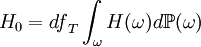
![S( k\delta t) = S(0) \exp( \Sigma_{i=0}^{i=k-1} [(\mu - \frac{\sigma^2}{2})\delta t + \sigma\epsilon_i\sqrt{\delta t}] )](images/math/3/6/9/3697358b622d7c8117809c7f9a180027.png)