To use all functions of this page, please activate cookies in your browser.
My watch list
my.chemeurope.com
my.chemeurope.com
With an accout for my.chemeurope.com you can always see everything at a glance – and you can configure your own website and individual newsletter.
- My watch list
- My saved searches
- My saved topics
- My newsletter
Ritz methodIn physics, the Ritz method is a variational method named after Walter Ritz. In quantum mechanics, a system of particles can be described in terms of an "energy functional" or Hamiltonian, which will measure the energy of any proposed configuration of said particles. It turns out that certain privileged configurations are more likely than other configurations, and this has to do with the eigenanalysis ("analysis of characteristics") of this Hamiltonian system. Because it is often impossible to analyze all of the infinite configurations of particles to find the one with the least amount of energy, it becomes essential to be able to approximate this Hamiltonian in some way for the purpose of numerical computations. The Ritz method can be used to achieve this goal. In the language of mathematics, it is exactly the finite element method used to compute the eigenvectors and eigenvalues of a Hamiltonian system. Product highlight
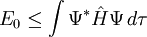
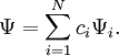
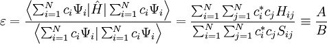
DiscussionAs with other variational methods, a trial wave function, Ψ, is tested on the system. This trial function is selected to meet boundary conditions (and any other physical constraints). The exact function is not known; the trial function contains one or more adjustable parameters, which are varied to find a lowest energy configuration. It can be shown that the ground state energy, E0, satisfies an inequality: that is, the ground-state energy is less than this value. The trial wave-function will always give an expectation value larger than the ground-energy (or at least, equal to it). If the trial wave function is known to be orthogonal to the ground state, then it will provide a boundary for the energy of some excited state. The Ritz ansatz function is a linear combination of N known basis functions With a known hamiltonian, we can write its expected value as
The basis functions are usually not orthogonal, so that the overlap matrix S has nonzero diagonal elements. Either
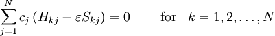
which leads to a set of N secular equations:
In the above equations, energy
which in turn is true only for N values of The relationship with the finite element methodIn the language of the finite element method, the matrix Hkj is precisely the stiffness matrix of the Hamiltonian in the piecewise linear element space, and the matrix Skj is the mass matrix. In the language of linear algebra, the value ε is an eigenvalue of the discretized Hamiltonian, and the vector c is a discretized eigenvector. PapersW. Ritz, "Ueber eine neue Methode zur Lösung gewisser Variationsprobleme der mathematischen Physik" J. Reine Angew. Math. 135 (1908 or 1909) 1 BooksCourant-Hilbert, p.157 See alsoSturm-Liouville theory |
|
| This article is licensed under the GNU Free Documentation License. It uses material from the Wikipedia article "Ritz_method". A list of authors is available in Wikipedia. |


 , parametrized by unknown coefficients:
 .
.
 or
or  (the conjugation of the first) can be used to minimize the expectation value. For instance, by making the partial derivatives of
  over
over 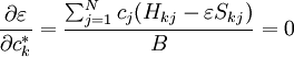 ,
,
 .
.
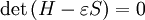
 are unknown. With respect to c, this is a homogeneous set of linear equations, which has a solution when the determinant of the coefficients to these unknowns is zero:
 ,
,
 will be real. The lowest value among
  , will be the best approximation to the ground state for the basis functions used. The remaining N-1 energies are estimates of excited state energies. An approximation for the wave function of state i can be obtained by finding the coefficients
 Last viewed


