To use all functions of this page, please activate cookies in your browser.
My watch list
my.chemeurope.com
my.chemeurope.com
With an accout for my.chemeurope.com you can always see everything at a glance – and you can configure your own website and individual newsletter.
- My watch list
- My saved searches
- My saved topics
- My newsletter
Solid harmonicsIn physics and mathematics, the solid harmonics are solutions of the Laplace equation in spherical polar coordinates. There are two kinds: the regular solid harmonics Product highlight
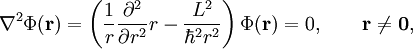
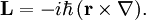
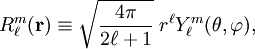
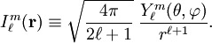
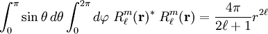
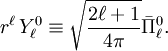
Derivation, relation to spherical harmonicsIntroducing r, θ, and φ for the spherical polar coordinates of the 3-vector r, we can write the Laplace equation in the following form where L2 is the square of the orbital angular momentum, It is known that spherical harmonics Yml are eigenfunctions of L2, Substitution of Φ(r) = F(r) Yml into the Laplace equation gives, after dividing out the spherical harmonic function, the following radial equation and its general solution, The particular solutions of the total Laplace equation are regular solid harmonics: and irregular solid harmonics: Racah's normalization (also known as Schmidt's semi-normalization) is applied to both functions (and analogously for the irregular solid harmonic) instead of normalization to unity. This is convenient because in many applications the Racah normalization factor appears unchanged throughout the derivations. Addition theoremsThe translation of the regular solid harmonic gives a finite expansion, where the Clebsch-Gordan coefficient is given by The similar expansion for irregular solid harmonics gives an infinite series, with ReferencesThe addition theorems were proved in different manners by many different workers. See for two different proofs for example:
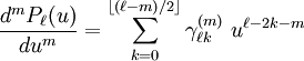
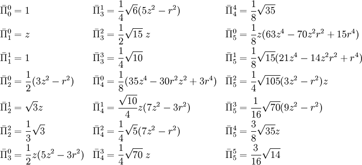
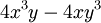
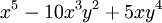
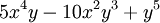
Real formBy a simple linear combination of solid harmonics of ±m these functions are transformed into real functions. The real regular solid harmonics, expressed in cartesian coordinates, are homogeneous polynomials of order l in x, y, z. The explicit form of these polynomials is of some importance. They appear, for example, in the form of spherical atomic orbitals and real multipole moments. The explicit cartesian expression of the real regular harmonics will now be derived. Linear combinationWe write in agreement with the earlier definition with where The following expression defines the real regular solid harmonics: and for m = 0: Since the transformation is by a unitary matrix the normalization of the real and the complex solid harmonics is the same. z-dependent partUpon writing u = cos θ the mth derivative of the Legendre polynomial can be written as the following expansion in u with Since z = r cosθ it follows that this derivative, times an appropriate power of r, is a simple polynomial in z, (x,y)-dependent partConsider next, recalling that x = r sinθcosφ and y = r sinθsinφ, Likewise Further and In totalList of lowest functionsWe list explicitly the lowest functions up to and including l = 5 .
Here The lowest functions
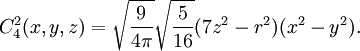
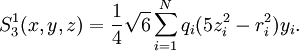
ExamplesThus, for example, the angular part of one of the nine normalized spherical g atomic orbitals is: One of the 7 components of a real multipole of order 3 (octupole) of a system of N charges qi is Spherical harmonics in Cartesian formThe following expresses normalized spherical harmonics in Cartesian coordinates (Condon-Shortley phase): and for m = 0: Here and for m > 0: For m = 0: ExamplesUsing the expressions for It may be verified that this agrees with the function listed here and here. |
||||||||||||||||||||||
| This article is licensed under the GNU Free Documentation License. It uses material from the Wikipedia article "Solid_harmonics". A list of authors is available in Wikipedia. |
 , which vanish at the origin and the irregular solid harmonics
  , which are singular at the origin. Both sets of functions play an important role in potential theory.


![L^2 Y^m_{\ell}\equiv \left[ L^2_x +L^2_y+L^2_z\right]Y^m_{\ell} = \ell(\ell+1) Y^m_{\ell}.](images/math/9/d/1/9d1436ba555cd04857277c3371c013c1.png)

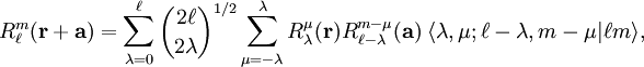
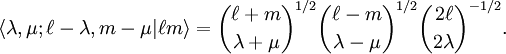

 . The quantity between pointed brackets is again a Clebsch-Gordan coefficient,


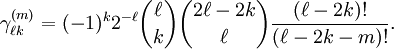
![\Theta_{\ell}^m (\cos\theta) \equiv \left[\frac{(\ell-m)!}{(\ell+m)!}\right]^{1/2} \,\sin^m\theta\, \frac{d^m P_\ell(\cos\theta)}{d\cos^m\theta}, \qquad m\ge 0,](images/math/0/2/a/02a77c91241732ba10a075902a0aec1c.png)
 is a Legendre polynomial of order l.
The m dependent phase is known as the
is a Legendre polynomial of order l.
The m dependent phase is known as the 

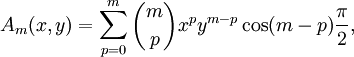
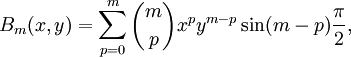
![r^m \sin^m\theta \cos m\varphi = \frac{1}{2} \left[ (r \sin\theta e^{i\varphi})^m + (r \sin\theta e^{-i\varphi})^m \right] = \frac{1}{2} \left[ (x+iy)^m + (x-iy)^m \right]](images/math/d/f/d/dfd1aea0e6f95b199e39761c6c8f0968.png)
![r^m \sin^m\theta \sin m\varphi = \frac{1}{2i} \left[ (r \sin\theta e^{i\varphi})^m - (r \sin\theta e^{-i\varphi})^m \right] = \frac{1}{2i} \left[ (x+iy)^m - (x-iy)^m \right].](images/math/8/5/d/85d42914755b1347970e19483b6d5915.png)
![A_m(x,y) \equiv \frac{1}{2} \left[ (x+iy)^m + (x-iy)^m \right]= \sum_{p=0}^m \binom{m}{p} x^p y^{m-p} \cos (m-p) \frac{\pi}{2}](images/math/3/a/2/3a25f7e174add17be597ee857ba82d65.png)
![B_m(x,y) \equiv \frac{1}{2i} \left[ (x+iy)^m - (x-iy)^m \right]= \sum_{p=0}^m \binom{m}{p} x^p y^{m-p} \sin (m-p) \frac{\pi}{2}.](images/math/3/9/6/396066928ca77a858c5f86eea8ab91d2.png)
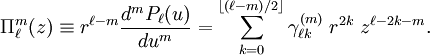
![C^m_\ell(x,y,z) = \left[\frac{(2-\delta_{m0}) (\ell-m)!}{(\ell+m)!}\right]^{1/2} \Pi^m_{\ell}(z)\;A_m(x,y),\qquad m=0,1, \ldots,\ell](images/math/4/2/8/428a7f7aff8aec77ae8b00ff442526fc.png)
![S^m_\ell(x,y,z) = \left[\frac{2 (\ell-m)!}{(\ell+m)!}\right]^{1/2} \Pi^m_{\ell}(z)\;B_m(x,y) ,\qquad m=1,2,\ldots,\ell.](images/math/d/b/6/db64065a519539ef5a9a3a26d49d0d0e.png)
![\bar{\Pi}^m_\ell(z) \equiv \left[\tfrac{(2-\delta_{m0}) (\ell-m)!}{(\ell+m)!}\right]^{1/2} \Pi^m_{\ell}(z) .](images/math/f/0/6/f0689759a40da2ffbed04aa8843d7255.png)
 and
and  are:
are:


![r^\ell\, \begin{pmatrix} Y_\ell^{m} \\ Y_\ell^{-m} \end{pmatrix} = \left[\frac{2\ell+1}{4\pi}\right]^{1/2} \bar{\Pi}^m_\ell \begin{pmatrix} (-1)^m (A_m + i B_m)/\sqrt{2} \\ \qquad (A_m - i B_m)/\sqrt{2} \\ \end{pmatrix} , \qquad m > 0.](images/math/2/f/8/2f82030a69c78c4a42351f69a4b58726.png)
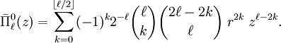
![\bar{\Pi}^m_\ell(z) = \left[\frac{(\ell-m)!}{(\ell+m)!}\right]^{1/2} \sum_{k=0}^{\left \lfloor (\ell-m)/2\right \rfloor} (-1)^k 2^{-\ell} \binom{\ell}{k}\binom{2\ell-2k}{\ell} \frac{(\ell-2k)!}{(\ell-2k-m)!} \; r^{2k}\; z^{\ell-2k-m}.](images/math/0/2/3/0232bce1152949a4eaea8a98e976c57d.png)
 ,
, ![Y^1_3 = - \frac{1}{r^3} \left[\tfrac{7}{4\pi}\cdot \tfrac{3}{16} \right]^{1/2} (5z^2-r^2)(x+iy) = - \left[\tfrac{7}{4\pi}\cdot \tfrac{3}{16}\right]^{1/2} (5\cos^2\theta-1) (\sin\theta e^{i\varphi})](images/math/0/1/a/01a36ea25d17997de3fc7af29efc835b.png)
![Y^{-2}_4 = \frac{1}{r^4} \left[\tfrac{9}{4\pi}\cdot\tfrac{5}{32}\right]^{1/2}(7z^2-r^2) (x-iy)^2 = \left[\tfrac{9}{4\pi}\cdot\tfrac{5}{32}\right]^{1/2}(7 \cos^2\theta -1) (\sin^2\theta e^{-2 i \varphi})](images/math/2/6/e/26e0b6b3459eb5f9c21c445ca7e4749a.png)


