To use all functions of this page, please activate cookies in your browser.
My watch list
my.chemeurope.com
my.chemeurope.com
With an accout for my.chemeurope.com you can always see everything at a glance – and you can configure your own website and individual newsletter.
- My watch list
- My saved searches
- My saved topics
- My newsletter
Constraint algorithmIn mechanics, a constraint algorithm is a method for satisfying constraints for bodies that obey Newton's equations of motion. There are three basic approaches to satisfying such constraints: choosing novel unconstrained coordinates ("internal coordinates"), introducing explicit constraint forces, and minimizing constraint forces implicitly by the technique of Lagrange multipliers or projection methods. Constraint algorithms are often applied to molecular dynamics simulations. Although such simulations are sometimes carried out in internal coordinates that automatically satisfy the bond-length and bond-angle constraints, they may also be carried out with explicit or implicit constraint forces for the bond lengths and bond angles. Explicit constraint forces typically shorten the time-step significantly, making the simulation less efficient computationally; in other words, more computer power is required to compute a trajectory of a given length. Therefore, internal coordinates and implicit-force constraint solvers are generally preferred. Additional recommended knowledge
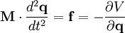
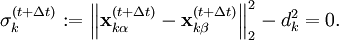
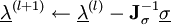
Mathematical backgroundThe motion of a set of N particles can be described by a set of second-order ordinary differential equations, Newton's second law, which can be written in matrix form where M is a mass matrix and q is the vector of generalized coordinates that describe the particles' positions. For example, the vector q may be a 3N Cartesian coordinates of the particle positions rk, where k runs from 1 to N; in the absence of constraints, M would be the 3Nx3N diagonal square matrix of the particle masses. The vector f represents the generalized forces and the scalar V(q) represents the potential energy, both of which are functions of the generalized coordinates q. If M constraints are present, the coordinates must also satisfy M time-independent algebraic equations where the index j runs from 1 to M. For brevity, these functions gi are grouped into an M-dimensional vector g below. The task is to solve the combined set of differential-algebraic (DAE) equations, instead of just the ordinary differential equations (ODE) of Newton's second law. This problem was studied in detail by Joseph Louis Lagrange, who laid out most of the methods for solving it.[1] The simplest approach is to define new generalized coordinates that are unconstrained; this approach eliminates the algebraic equations and reduces the problem once again to solving an ordinary differential equation. Such an approach is used, for example, in describing the motion of a rigid body; the position and orientation of a rigid body can be described by six independent, unconstrained coordinates, rather than describing the positions of the particles that make it up and the constraints among them that maintain their relative distances. The drawback of this approach is that the equations may become unwieldy and complex; for example, the mass matrix M may become non-diagonal and depend on the generalized coordinates. A second approach is to introduce explicit forces that work to maintain the constraint; for example, one could introduce strong spring forces that enforce the distances among mass points within a "rigid" body. The two difficulties of this approach are that the constraints are not satisfied exactly, and the strong forces may require very short time-steps, making simulations inefficient computationally. A third approach is to use a method such as Lagrange multipliers or projection to the constraint manifold to determine the coordinate adjustments necessary to satisfy the constraints. Finally, there are various hybrid approaches in which different sets of constraints are satisfied by different methods, e.g., internal coordinates, explicit forces and implicit-force solutions. Internal coordinate methodsThe simplest approach to satisfying constraints in energy minimization and molecular dynamics is to represent the mechanical system in so-called internal coordinates corresponding to unconstrained independent degrees of freedom of the system. For example, the dihedral angles of a protein are an independent set of coordinates that specify the positions of all the atoms without requiring any constraints. The difficulty of such internal-coordinate approaches is twofold: the Newtonian equations of motion become much more complex and the internal coordinates may be difficult to define for cyclic systems of constraints, e.g., in ring puckering or when a protein has a disulfide bond. The original methods for efficient recursive energy minimization in internal coordinates were developed by Gō and coworkers.[2][3] Efficient recursive, internal-coordinate constraint solvers were extended to molecular dynamics.[4][5] Analogous methods were applied later to other systems.[6][7][8] Lagrange multiplier-based methodsIn most molecular dynamics simulation, constraints are enforced using the method of Lagrange multipliers. Given a set of n linear (holonomic) constraints at the time t, where These constraint equations, are added to the potential energy function in the equations of motion, resulting in, for each of the N particles in the system Adding the constraint equations to the potential does not change it, since all Integrating both sides of the equations of motion twice in time yields the constrained particle positions at the time t + Δt where To satisfy the constraints This implies solving a systen of n non-linear equations simultaneously for the n unknown Lagrange multipliers λk. This system of n non-linear equations in n unknowns is best solved using Newton's method where the solution vector where Since not all particles are involved in all constraints, Furthermore, instead of constantly updating the vector
The vector is then reset to This is repeated until the constraint equations Although there are a number of algorithms to compute the Lagrange multipliers, they differ only in how they solve the system of equations, usually using Quasi-Newton methods. The SETTLE algorithmThe SETTLE algorithm[9] solves the system of non-linear equations analytically for n = 3 constraints in constant time. Although it does not scale to larger numbers of constraints, it is very often used to constrain rigid water molecules, which are present in almost all biological simulations and are usually modelled using three constraints (e.g. SPC/E and TIP3P water models). The SHAKE algorithmThe SHAKE algorithm was the first algorithm developed to satisfy bond geometry constraints during molecular dynamics simulations.[10] It solves the system of non-linear constraint equations using the Gauss-Seidel method to approximate the solution of the linear system of equations in the Newton iteration. This amounts to assuming that
for all Each iteration of the SHAKE algorithm costs A noniterative form of SHAKE was developed later.[11] Several variants of the SHAKE algorithm exist. Although they differ in how they compute or apply the constraints themselves, the constraints are still modelled using Lagrange multipliers which are computed using the Gauss-Seidel method. The original SHAKE algorithm is limited to mechanical systems with a tree structure, i.e., no closed loops of constraints. A later extension of the method, QSHAKE (Quaternion SHAKE) was developed to amend this.[12] It works satisfactorily for rigid loops such as aromatic ring systems but fails for flexible loops, such as when a protein has a disulfide bond.[13] Further extensions include RATTLE[14], WIGGLE[15] and MSHAKE[16]. RATTLE works the same way as SHAKE, yet using the Velocity Verlet time integration scheme. WIGGLE extends SHAKE and RATTLE by using an initial estimate for the Lagrange multipliers λk based on the particle velocities. Finally, MSHAKE computes corrections on the constraint forces, achieving better convergence. A final modification is the P-SHAKE algorithm[17] for rigid or semi-rigid molecules. P-SHAKE computes and updates a pre-conditioner which is applied to the constraint gradients before the SHAKE iteration, causing the Jacobian The M-SHAKE algorithmThe M-SHAKE algorithm[18] solves the non-linear system of equations using Newton's method directly. In each iteration, the linear system of equations is solved exactly using an LU decomposition. Each iteration costs This solution was first proposed in 1986 by Ciccotti and Ryckaert[19] under the title "the matrix method", yet differed in the solution of the linear system of equations. Ciccotti and Ryckaert suggest inverting the matrix The LINCS algorithmAn alternative constraint method, LINCS (Linear Constraint Solver) was developed in 1997,[20] but was based on earlier method, EEM,[21] and a modification thereof.[22] LINCS has been reported to be 3-4 times faster than SHAKE.[20] LINCS applies Lagrange multipliers to the constraint forces and solves for the multipliers by using a series expansion to approximate the inverse of the Jacobian in each step of the Newton iteration. The inversion only works for matrices with Eigenvalues smaller than 1, making the algorithm suitable only for molecules with low connectivity. Hybrid methodsHybrid methods have also been introduced in which the constraints are divided into two groups; the constraints of the first group are solved using internal coordinates whereas those of the second group are solved using constraint forces, e.g., by a Lagrange multiplier or projection method.[23][24][25] This approach was pioneered by Lagrange,[1] and result in Lagrange equations of the mixed type.[26] See alsoReferences and footnotes
Categories: Molecular dynamics | Computational chemistry | Molecular physics |
||||||||||
| This article is licensed under the GNU Free Documentation License. It uses material from the Wikipedia article "Constraint_algorithm". A list of authors is available in Wikipedia. |


 and
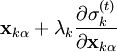
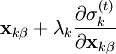
and  are the positions of the two particles involved in the kth constraint at the time t and
 ![\frac{\partial^2 \mathbf x_i^{(t)}}{\partial t^2} m_i = \frac{\partial}{\partial \mathbf x_i} \left[ V(\mathbf x_i^{(t)}) + \sum_{k=1}^n \lambda_k \sigma_k^{(t)} \right], \quad i=1 \dots N.](images/math/f/b/6/fb696721a7d7d1090ee87956c274f79d.png)
 should, ideally, be zero.
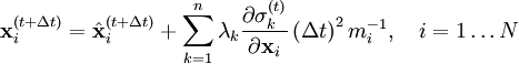
 is the unconstrained (or uncorrected) position of the ith particle after integrating the unconstrained equations of motion.
 in the next timestep, the Lagrange multipliers must be chosen such that
![\sigma_j^{(t + \Delta t)} := \left\| \hat{\mathbf x}_{j\alpha}^{(t+\Delta t)} - \hat{\mathbf x}_{j\beta}^{(t+\Delta t)} + \sum_{k=1}^n \lambda_k \left[ \frac{\partial\sigma_k^{(t)}}{\partial \mathbf x_{j\alpha}}m_{j\alpha}^{-1} - \frac{\partial\sigma_k^{(t)}}{\partial \mathbf x_{j\beta}}m_{j\beta}^{-1}\right] \right\|_2^2 - d_k^2 = 0, \quad j = 1 \dots n](images/math/e/8/1/e812c2179ef30beb4a7141c3ede4a8e7.png)
 is updated using
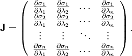
 is the Jacobian of the equations σk:
 , resulting in simpler expressions for
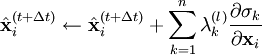
  . After each iteration, the unconstrained particle positions are updated using
 .
.


 iteratively until the constraint equations
  operations and the iterations themselves converge linearly.
 .
.
 operations, yet the solution converges quadratically, requiring much less iterations than SHAKE.


