To use all functions of this page, please activate cookies in your browser.
My watch list
my.chemeurope.com
my.chemeurope.com
With an accout for my.chemeurope.com you can always see everything at a glance – and you can configure your own website and individual newsletter.
- My watch list
- My saved searches
- My saved topics
- My newsletter
AdvectionAdvection is transport in a fluid. The fluid is described mathematically for such processes as a vector field, and the material transported is described as a scalar concentration of substance, which is present in the fluid. A good example of advection is the transport of pollutants or silt in a river: the motion of the water carries these impurities downstream. Another commonly advected substance is heat, and here the fluid may be water, air, or any other heat-containing fluid material. Any substance, or conserved property (such as heat) can be advected, in a similar way, in any fluid. Advection is important for the formation of orographic cloud and the precipitation of water from clouds, as part of the hydrological cycle. In meteorology and physical oceanography, advection often refers to the transport of some property of the atmosphere or ocean, such as heat, humidity (see moisture) or salinity. Meteorological or oceanographic advection follows isobaric surfaces and is therefore predominantly horizontal. Product highlight
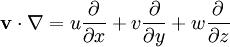
MeteorologyIn meteorology and physical oceanography, advection often refers to the transport of some property of the atmosphere or ocean, such as heat, humidity (see moisture) or salinity. Meteorological or oceanographic advection follows isobaric surfaces and is therefore predominantly horizontal. Advection is important for the formation of orographic cloud and the precipitation of water from clouds, as part of the hydrological cycle. Other quantitiesThe advection equation also applies if the quantity being advected is represented by a probability density function at each point, although accounting for diffusion is more difficult. Mathematics of advectionThe advection equation is the partial differential equation that governs the motion of a conserved scalar as it is advected by a known velocity field. It is derived using the scalar's conservation law, together with Gauss's theorem, and taking the infinitesimal limit. Perhaps the best image to have in mind is the transport of salt dumped in a river. If the river is originally fresh water and is flowing quickly, the predominant form of transport of the salt in the water will be advective, as the water flow itself would transport the salt. If the river was not flowing the salt would simply disperse outwards from its source in a diffusive manner, which is not advection. In Cartesian coordinates the advection operator is
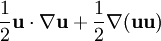
where the velocity vector v has components u, v and w in the x, y and z directions respectively. The advection equation for a scalar ψ, such as temperature, is expressed mathematically as: where For a vector In particular, if the flow is steady, The advection equation is not simple to solve numerically: the system is a hyperbolic partial differential equation, and interest typically centers on discontinuous "shock" solutions (which are notoriously difficult for numerical schemes to handle). Even in one space dimension and constant velocity, the system remains difficult to simulate. The equation becomes where ψ = ψ(x,t) is the scalar being advected and u the x component of the vector According to [1], numerical simulation can be aided by considering the skew symmetric form for the advection operator. where Since skew symmetry implies only complex eigenvalues, this form reduces the "blow up" and "spectral blocking" often experienced in numerical solutions with sharp discontinuities (see Boyd [2]) See also
References
Categories: Equations of fluid dynamics | Convection |
|
| This article is licensed under the GNU Free Documentation License. It uses material from the Wikipedia article "Advection". A list of authors is available in Wikipedia. |


 .
.
 is the divergence operator and
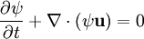
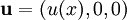
  is the vector field. Frequently, it is assumed that the velocity field is
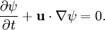
  . If this is so, the above equation reduces to
 , such as magnetic field or velocity, in a solenoidal field it is defined as:
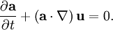
 which shows that
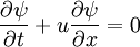
 .
.
 is a vector with components
 ![[\nabla ({\bold u} u_x),\nabla ({\bold u} u_y),\nabla ({\bold u} u_z)]](images/math/1/5/e/15e7a5e1ee835b0df6691f9df8fd7747.png) and the notation
and the notation ![{\bold u} = [u_x,u_y,u_z]](images/math/f/5/f/f5f0c9d3a9287052061eb083369fc8d2.png) has been used.
has been used.
Last viewed


