To use all functions of this page, please activate cookies in your browser.
My watch list
my.chemeurope.com
my.chemeurope.com
With an accout for my.chemeurope.com you can always see everything at a glance – and you can configure your own website and individual newsletter.
- My watch list
- My saved searches
- My saved topics
- My newsletter
Associated Legendre function
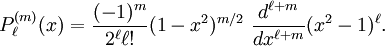
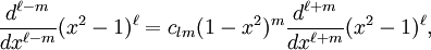
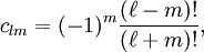
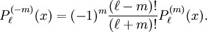
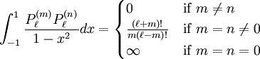
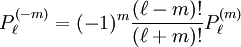
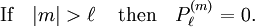
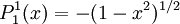
In mathematics, the associated Legendre functions are the canonical solutions of the general Legendre equation or where the indices This ordinary differential equation is frequently encountered in physics and other technical fields. In particular, it occurs when solving Laplace's equation (and related partial differential equations) in spherical coordinates. Product highlightDefinitionThese functions are denoted The ( − 1)m factor in this formula is known as the Condon-Shortley phase. Some authors omit it. Since, by Rodrigues' formula, one obtains This equation allows extension of the range of m to: -l ≤ m ≤ l. The definitions of Pl(±m), resulting from this expression by substitution of ±m, are proportional. Indeed, equate the coefficients of equal powers on the left and right hand side of then it follows that the proportionality constant is so that OrthogonalityAssuming Where Also, they satisfy the orthogonality condition for fixed Negative m and/or negative lThe differential equation is clearly invariant under a change in sign of m. The functions for negative m were shown above to be proportional to those of positive m: (This followed from the Rodrigues' formula definition. This definition also makes the various recurrence formulas work for positive or negative m.)
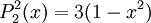
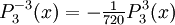
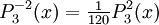
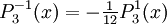
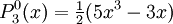
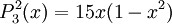
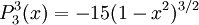
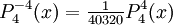
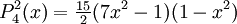
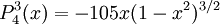
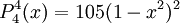
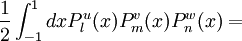
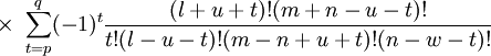
The differential equation is also invariant under a change from The first few associated Legendre polynomialsThe first few associated Legendre polynomials, including those for negative values of m, are: Recurrence formulaeThese functions have a number of recurrence properties: Gaunt's formulaThe integral over the product of three associated Legendre polynomials (with orders matching as shown below) turns out to be necessary when doing atomic calculations of the Hartree-Fock variety where matrix elements of the Coulomb operator are needed. For this we have Gaunt's formula [1]
This formula is to be used under the following assumptions:
Other quantities appearing in the formula are defined as
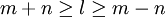
The integral is zero unless
The Legendre functions, and the hypergeometric functionThese functions may be defined for general complex parameters and argument: where Γ is the gamma function and so that They are called the Legendre functions when defined in this more general way. They satisfy the same differential equation as before: Since this is a second order differential equation, it has a second solution,
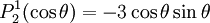
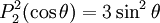
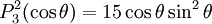
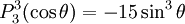
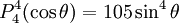
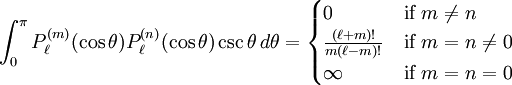
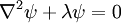
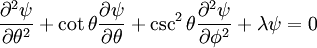
Reparameterization in terms of anglesThese functions are most useful when the argument is reparameterized in terms of angles, letting x = cosθ: The first few polynomials, parameterized this way, are: For fixed m, Also, for fixed In terms of θ, More precisely, given an integer m Applications in physics: Spherical harmonicsIn many occasions in physics, associated Legendre polynomials in terms of angles occur where spherical symmetry is involved. The colatitude angle in spherical coordinates is the angle θ used above. The longitude angle, φ, appears in a multiplying factor. Together, they make a set of functions called spherical harmonics. These functions express the symmetry of the two-sphere under the action of the Lie group SO(3). As such, Legendre polynomials can be generalized to express the symmetries of semi-simple Lie groups and Riemannian symmetric spaces. What makes these functions useful is that they are central to the solution of the equation
When the partial differential equation is solved by the method of separation of variables, one gets a φ-dependent part sin(mφ) or cos(mφ) for integer m≥0, and an equation for the θ-dependent part for which the solutions are Therefore, the equation has nonsingular separated solutions only when and For each choice of The solutions are usually written in terms of complex exponentials: The functions The spherical harmonic functions form a complete orthonormal set of functions in the sense of Fourier series. It should be noted that workers in the fields of geodesy, geomagnetism and spectral analysis use a different phase and normalization factor than given here (see spherical harmonics). When a 3-dimensional spherically symmetric partial differential equation is solved by the method of separation of variables in spherical coordinates, the part that remains after removal of the radial part is typically
of the form See also
Notes
References
|
||||
| This article is licensed under the GNU Free Documentation License. It uses material from the Wikipedia article "Associated_Legendre_function". A list of authors is available in Wikipedia. |
 and m—are commonly called "associated Legendre polynomials", even though they are not polynomials when m is odd. The fully general class of functions described here, with arbitrary real or complex values of
  and m, are sometimes called "generalized Legendre functions", or just "Legendre functions". In that case the parameters are usually renamed with Greek letters.
![(1-x^2)\,y'' -2xy' + \left(\ell[\ell+1] - \frac{m^2}{1-x^2}\right)\,y = 0,\,](images/math/0/2/3/02361edfec94abdc3c0d8368110cdd60.png)
![([1-x^2]\,y')' + \left(\ell[\ell+1] - \frac{m^2}{1-x^2}\right)\,y = 0,\,](images/math/3/b/0/3b021eaa11ac4f85730fa37e9a412895.png)


 . We put the superscript in parentheses
to avoid confusing it with an exponent. Their most straightforward definition is in terms
of derivatives of ordinary Legendre polynomials (m ≥ 0)
. We put the superscript in parentheses
to avoid confusing it with an exponent. Their most straightforward definition is in terms
of derivatives of ordinary Legendre polynomials (m ≥ 0)
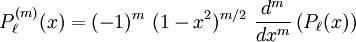
![P_\ell(x) = \frac{1}{2^\ell\,\ell!} \ \frac{d^\ell}{dx^\ell}\left([x^2-1]^\ell\right),](images/math/a/8/8/a8808c5457ef37f07d3d96075c212ff3.png)
 , they satisfy the orthogonality condition for fixed m:
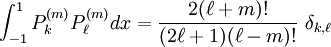
 is the Kronecker delta.
 , and the functions for negative


![P_{\lambda}^{(\mu)}(z) = \frac{1}{\Gamma(1-\mu)} \left[\frac{1+z}{1-z}\right]^{\mu/2} \,_2F_1 (-\lambda, \lambda+1; 1-\mu; \frac{1-z}{2})](images/math/2/e/b/2ebc03d81f4dbccf8e371da9c40aabae.png)
 is the hypergeometric function
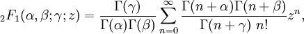
![P_{\lambda}^{(\mu)}(z) = \frac{1}{\Gamma(-\lambda)\Gamma(\lambda+1)} \left[\frac{1+z}{1-z}\right]^{\mu/2} \sum_{n=0}^\infty\frac{\Gamma(n-\lambda)\Gamma(n+\lambda+1)}{\Gamma(n+1-\mu)\ n!}\left(\frac{1-z}{2}\right)^n.](images/math/e/9/9/e99114974478e326ac8c93330f55a259.png)
![(1-z^2)\,y'' -2zy' + \left(\lambda[\lambda+1] - \frac{\mu^2}{1-z^2}\right)\,y = 0.\,](images/math/c/5/2/c525aadad3aa5e5456bad5729e8e75c5.png)
 , defined as:

 and
and 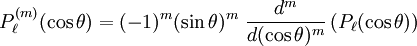


 are orthogonal, parameterized by θ over
![\frac{d^{2}y}{d\theta^2} + \cot \theta \frac{dy}{d\theta} + \left[\lambda - \frac{m^2}{\sin^2\theta}\right]\,y = 0\,](images/math/f/0/7/f0750ee5012238f5c7e86dde781128c4.png)
 0, the above equation has
nonsingular solutions only when
0, the above equation has
nonsingular solutions only when  for
for  , and those solutions are proportional to
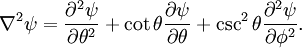
 on the surface of a sphere. In spherical coordinates θ (colatitude) and φ (longitude), the Laplacian is
 and
and 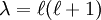 .
.


 functions
for the various values of m and choices of sine and cosine.
They are all orthogonal in both
functions
for the various values of m and choices of sine and cosine.
They are all orthogonal in both 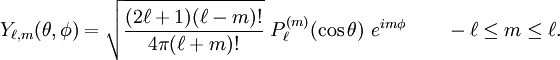
 are the
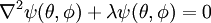 , and hence the solutions are spherical harmonics.


