To use all functions of this page, please activate cookies in your browser.
My watch list
my.chemeurope.com
my.chemeurope.com
With an accout for my.chemeurope.com you can always see everything at a glance – and you can configure your own website and individual newsletter.
- My watch list
- My saved searches
- My saved topics
- My newsletter
Spherical harmonicsIn mathematics, the spherical harmonics are the angular portion of an orthogonal set of solutions to Laplace's equation represented in a system of spherical coordinates. Spherical harmonics are important in many theoretical and practical applications, particularly in the computation of atomic electron configurations, the representation of the gravitational field, geoid, and magnetic field of planetary bodies, characterization of the cosmic microwave background radiation. In 3D computer graphics, spherical harmonics plays a special role in a wide variety of topics including indirect lighting (ambient occlusion, global illumination, precomputed radiance transfer etc) and in recognition of 3D shapes. Product highlight
Introduction
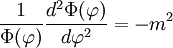
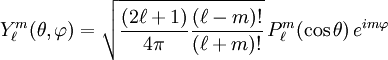
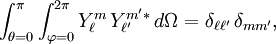
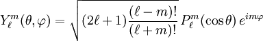
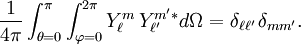
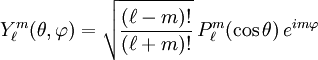
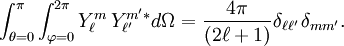
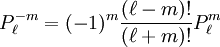
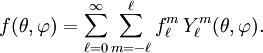
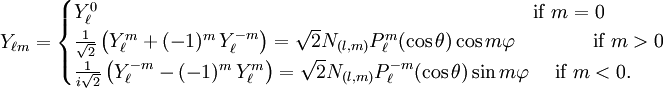
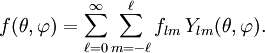
Laplace's equation in spherical coordinates is: (see also del in cylindrical and spherical coordinates). For f(r,θ,φ)=R(r)Θ(θ)Φ(φ), the angular portion of Laplace's equation satisfies Using the technique of separation of variables, two differential equations result: for some m and l. Hence, the angular solutions can be shown to be a products of trigonometric functions and associated Legendre functions: where When Laplace's equation is solved on the surface of the sphere, the periodic boundary conditions in φ, as well as regularity conditions at both the north and south poles, ensure that the degree where Orthogonality and normalizationSeveral different normalizations are in common use for the spherical harmonic functions. In physics and seismology, these functions are generally defined as which are orthonormal where δaa = 1, δab = 0 if a ≠ b, (see Kronecker delta) and dΩ = sinθ dφ dθ. The disciplines of geodesy and spectral analysis use which possess unit power The magnetics community, in contrast, uses Schmidt semi-normalized harmonics which have the normalization In quantum mechanics this normalization is often used, too, and is there named Racah's normalization after Giulio Racah. Using the identity (see associated Legendre functions) it can be shown that all of the above normalized spherical harmonic functions satisfy where the superscript * denotes complex conjugation. Alternatively, this equation follows from the relation of the spherical harmonic functions with the Wigner D-matrix. Condon-Shortley phaseOne source of confusion with the definition of the spherical harmonic functions concerns a phase factor of (-1)m, commonly referred to as the Condon-Shortley phase in the quantum mechanical literature. In the quantum mechanics community, it is common practice to either include this phase factor in the definition of the associated Legendre functions, or to append it to the definition of the spherical harmonic functions. There is no requirement to use the Condon-Shortley phase in the definition of the spherical harmonic functions, but including it can simplify some quantum mechanical operations, especially the application of raising and lowering operators. The geodesy and magnetics communities never include the Condon-Shortley phase factor in their definitions of the spherical harmonic functions. Spherical harmonics expansionThe spherical harmonics form a complete set of orthonormal functions and thus form a vector space analogous to unit basis vectors. On the unit sphere, any square-integrable function can thus be expanded as a linear combination of these:
This expansion is exact as long as
An alternative set of spherical harmonics for real functions may be obtained by taking the set:
where N(l,m) denotes the normalization constant as a function of l and m. These functions have the same normalization properties as the complex ones above. In this notation, a real square-integrable function can be expressed as an infinite sum of real spherical harmonics as:
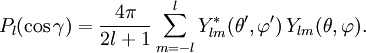
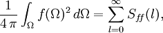
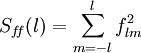
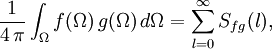
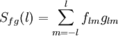
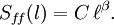
See here for a list of real spherical harmonics up to and including l = 5. Note, however, that the listed functions differ by the phase (-1)m from the phase given in this article. Spectrum analysisThe total power of a function f is defined in the signal processing literature as the integral of the function squared, divided by the area it spans. Using the orthonormality properties of the real unit-power spherical harmonic functions, it is straightforward to verify that the total power of a function defined on the unit sphere is related to its spectral coefficients by a generalization of Parseval's theorem: where is defined as the angular power spectrum. In a similar manner, one can define the cross-power of two functions as where is defined as the cross-power spectrum. If the functions f and g have a zero mean (i.e., the spectral coefficients f00 and g00 are zero), then Sff(l) and Sfg(l) represent the contributions to the function's variance and covariance for degree When β = 0, the spectrum is "white" as each degree possesses equal power. When β < 0, the spectrum is termed "red" as there is more power at the low degrees with long wavelengths than higher degrees. Finally, when β > 0, the spectrum is termed "blue". Addition theoremA mathematical result of considerable interest and use is called the addition theorem for spherical harmonics. Two vectors r and r', with spherical coordinates The addition theorem expresses a Legendre polynomial of order l in the angle
This expression is valid for both real and complex harmonics. However, it should be emphasized that the quoted form above is valid only for the orthonormalized spherical harmonics. For unit power harmonics it is only necessary to remove the factor of 4π. Visualization of the spherical harmonics
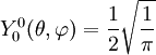
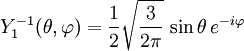
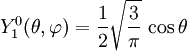
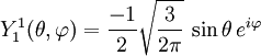
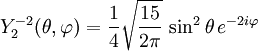
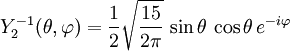
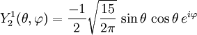
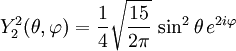
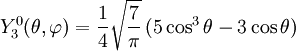
The spherical harmonics are easily visualized by counting the number of zero crossings they possess in both the latitudinal and longitudinal directions. For the latitudinal direction, the associated Legendre functions possess l − | m | zeros, whereas for the longitudinal direction, the trigonomentric sin and cos functions possess 2 | m | zeros. When the spherical harmonic order m is zero, the spherical harmonic functions do not depend upon longitude, and are referred to as zonal. When l = | m | , there are no zero crossings in latitude, and the functions are referred to as sectoral. For the other cases, the functions checker the sphere, and they are referred to as tesseral. First few spherical harmonicsAnalytic expressions for the first few orthonormalized spherical harmonics that use the Condon-Shortley phase convention:
GeneralizationsThe spherical harmonics map can be seen as representations of the symmetry group of rotations around a point (SO(3)) and its double-cover SU(2). As such they capture the symmetry of the two-dimensional sphere (or two-sphere). Each set of spherical harmonics with a given value for the l-parameter map onto a different irreducible representation of SO(3). In addition, the two-sphere is equivalent to the Riemann sphere. The complete set of symmetries of the Riemann sphere are described by the Mobius transformation group PSL(2,C), which is isomorphic as a real Lie group to the Lorentz group. The analog of the spherical harmonics for the Lorentz group are given by the hypergeometric series; indeed, the spherical harmonics can be re-expressed in terms of the hypergeometric series, as SO(3) is a subgroup of PSL(2,C). More generally, hypergeometric series can be generalized to describe the symmetries of any symmetric space; in particular, hypergeometric series can be developed for any Lie group[1][2][3][4] See also
ReferencesCited references
General references
Web resources
Software
|
|
| This article is licensed under the GNU Free Documentation License. It uses material from the Wikipedia article "Spherical_harmonics". A list of authors is available in Wikipedia. |


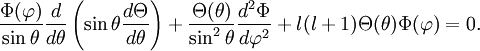
![l(l+1)\sin ^2(\theta) + \frac{\sin(\theta)}{\Theta(\theta)} \frac{d}{d\theta} \left [ \sin(\theta) \frac{d\Theta}{d\theta} \right ] = m^2](images/math/a/3/4/a34e5fe43543df9c4cfefadaf94e7b6b.png)

 is a called a spherical harmonic function of degree
  and order m,
  is an
is an 
 and
and  are constants. The terms in the first summation approach zero as r goes to infinity, whereas the terms in the second summation approach zero at the origin.

 , and utilizing the above orthogonality relationships. For the case of orthonormalized harmonics, this gives:

 and
and  ,respectively, have an angle
  between them given by

 and
and  :
: