To use all functions of this page, please activate cookies in your browser.
My watch list
my.chemeurope.com
my.chemeurope.com
With an accout for my.chemeurope.com you can always see everything at a glance – and you can configure your own website and individual newsletter.
- My watch list
- My saved searches
- My saved topics
- My newsletter
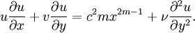
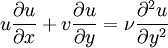
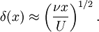
Blasius boundary layerA Blasius boundary layer, in physics and fluid mechanics, describes the steady two-dimensional boundary layer that forms on a semi-infinite plate which is held parallel to a constant unidirectional flow U. Product highlightWithin the boundary layer the usual balance between viscosity and convective inertia is struck, resulting in the scaling argument
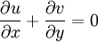
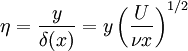
where δ is the boundary-layer thickness and ν is the kinematic viscosity. However the semi-infinite plate has no natural length scale L and so the steady, two-dimensional boundary-layer equations (note that the x-independence of U has been accounted for in the boundary-layer equations) admit a similarity solution. In the system of partial differential equations written above it is assumed that a fixed solid body wall is parallel to the x-direction whereas the y-direction is normal with respect to the fixed wall. u and v denote here the x- and y-components of the fluid velocity vector. Furthermore, from the scaling argument it is apparent that the boundary layer grows with the downstream coordinate x, e.g. This suggests adopting the similarity variable and writing
It proves convenient to work with the stream function ψ, in which case
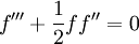
and on differentiating, to find the velocities, and substituting into the boundary-layer equation we obtain the Blasius equation subject to
f = f' = 0 on η = 0 and
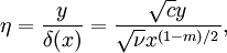
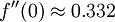
can then be computed. The numerical solution gives Falkner-Skan boundary layerA generalisation of the Blasius boundary layer that considers outer flows of the form U = cxm results in a boundary-layer equation of the form Under these circumstances the appropriate similarity variable becomes
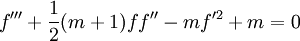
and, as in the Blasius boundary layer, it is convenient to use a stream function ψ = U(x)δ(x)f(η) = cxmδ(x)f(η) This results in the Falkner-Skan equation
(note that m = 0 produces the Blasius equation). References
|
| This article is licensed under the GNU Free Documentation License. It uses material from the Wikipedia article "Blasius_boundary_layer". A list of authors is available in Wikipedia. |


 ,
,
 as
as  . This non-linear ODE must be solved numerically, with the shooting method proving an effective choice.
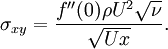
The shear stress on the plate
. This non-linear ODE must be solved numerically, with the shooting method proving an effective choice.
The shear stress on the plate
 .
.