To use all functions of this page, please activate cookies in your browser.
My watch list
my.chemeurope.com
my.chemeurope.com
With an accout for my.chemeurope.com you can always see everything at a glance – and you can configure your own website and individual newsletter.
- My watch list
- My saved searches
- My saved topics
- My newsletter
Viscosity
Viscosity is a measure of the resistance of a fluid to being deformed by either shear stress or extensional stress. It is commonly perceived as "thickness", or resistance to flow. Viscosity describes a fluid's internal resistance to flow and may be thought of as a measure of fluid friction. Thus, water is "thin", having a lower viscosity, while vegetable oil is "thick" having a higher viscosity. All real fluids (except superfluids) have some resistance to stress, but a fluid which has no resistance to shear stress is known as an ideal fluid or inviscid fluid.[1] The study of viscosity is known as rheology. Product highlightEtymologyThe word "viscosity" derives from the Latin word "viscum" for mistletoe. A viscous glue was made from mistletoe berries and used for lime-twigs to catch birds.[2] Viscosity coefficientsWhen looking at a value for viscosity, the number that one most often sees is the coefficient of viscosity. There are several different viscosity coefficients depending on the nature of applied stress and nature of the fluid. They are introduced in the main books on hydrodynamics[3][4] and rheology.[5]
Shear viscosity and dynamic viscosity are much better known than the others. That is why they are often referred to as simply viscosity. Simply put, this quantity is the ratio between the pressure exerted on the surface of a fluid, in the lateral or horizontal direction, to the change in velocity of the fluid as you move down in the fluid (this is what is referred to as a velocity gradient). For example, at "room temperature", water has a nominal viscosity of 1.0 × 10⁻³ Pa∙s and motor oil has a nominal apparent viscosity of 250 × 10-3 Pa∙s.[6]
Newton's theory
In general, in any flow, layers move at different velocities and the fluid's viscosity arises from the shear stress between the layers that ultimately opposes any applied force. Isaac Newton postulated that, for straight, parallel and uniform flow, the shear stress, τ, between layers is proportional to the velocity gradient, ∂u/∂y, in the direction perpendicular to the layers.
Here, the constant η is known as the coefficient of viscosity, the viscosity, the dynamic viscosity, or the Newtonian viscosity. Many fluids, such as water and most gases, satisfy Newton's criterion and are known as Newtonian fluids. Non-Newtonian fluids exhibit a more complicated relationship between shear stress and velocity gradient than simple linearity. The relationship between the shear stress and the velocity gradient can also be obtained by considering two plates closely spaced apart at a distance y, and separated by a homogeneous substance. Assuming that the plates are very large, with a large area A, such that edge effects may be ignored, and that the lower plate is fixed, let a force F be applied to the upper plate. If this force causes the substance between the plates to undergo shear flow (as opposed to just shearing elastically until the shear stress in the substance balances the applied force), the substance is called a fluid. The applied force is proportional to the area and velocity of the plate and inversely proportional to the distance between the plates. Combining these three relations results in the equation F = η(Au/y), where η is the proportionality factor called the absolute viscosity (with units Pa·s = kg/(m·s) or slugs/(ft·s)). The absolute viscosity is also known as the dynamic viscosity, and is often shortened to simply viscosity. The equation can be expressed in terms of shear stress; τ = F/A = η(u/y). The rate of shear deformation is u / y and can be also written as a shear velocity, du/dy. Hence, through this method, the relation between the shear stress and the velocity gradient can be obtained. James Clerk Maxwell called viscosity fugitive elasticity because of the analogy that elastic deformation opposes shear stress in solids, while in viscous fluids, shear stress is opposed by rate of deformation. Viscosity MeasurementDynamic viscosity is measured with various types of viscometer. Close temperature control of the fluid is essential to accurate measurements, particularly in materials like lubricants, whose viscosity can double with a change of only 5 °C. For some fluids, it is a constant over a wide range of shear rates. These are Newtonian fluids. The fluids without a constant viscosity are called Non-Newtonian fluids. Their viscosity cannot be described by a single number. Non-Newtonian fluids exhibit a variety of different correlations between shear stress and shear rate. One of the most common instruments for measuring kinematic viscosity is the glass capillary viscometer. In paint industries, viscosity is commonly measured with a Zahn cup, in which the efflux time is determined and given to customers. The efflux time can also be converted to kinematic viscosities (cSt) through the conversion equations. Also used in paint, a Stormer viscometer uses load-based rotation in order to determine viscosity. The viscosity is reported in Krebs units (KU), which are unique to Stormer viscometers. Vibrating viscometers can also be used to measure viscosity. These models use vibration rather than rotation to measure viscosity. Extensional viscosity can be measured with various rheometers that apply extensional stress Volume viscosity can be measured with acoustic rheometer. Units of MeasureViscosity (dynamic/absolute viscosity)Dynamic viscosity and absolute viscosity are synonymous. The IUPAC symbol for viscosity is the Greek symbol eta (η), and dynamic viscosity is also commonly referred to using the Greek symbol mu (μ). The SI physical unit of dynamic viscosity is the pascal-second (Pa·s), which is identical to 1 kg·m−1·s−1. If a fluid with a viscosity of one Pa·s is placed between two plates, and one plate is pushed sideways with a shear stress of one pascal, it moves a distance equal to the thickness of the layer between the plates in one second. The name poiseuille (Pl) was proposed for this unit (after Jean Louis Marie Poiseuille who formulated Poiseuille's law of viscous flow), but not accepted internationally. Care must be taken in not confusing the poiseuille with the poise named after the same person. The cgs physical unit for dynamic viscosity is the poise[8] (P), named after Jean Louis Marie Poiseuille. It is more commonly expressed, particularly in ASTM standards, as centipoise (cP). The centipoise is commonly used because water has a viscosity of 1.0020 cP (at 20 °C; the closeness to one is a convenient coincidence).
The relation between poise and pascal-seconds is:
Kinematic viscosityIn many situations, we are concerned with the ratio of the viscous force to the inertial force, the latter characterised by the fluid density ρ. This ratio is characterised by the kinematic viscosity (ν), defined as follows:
where μ is the (dynamic) viscosity, and ρ is the density. Kinematic viscosity (Greek symbol: ν) has SI units (m2·s−1). The cgs physical unit for kinematic viscosity is the stokes (abbreviated S or St), named after George Gabriel Stokes. It is sometimes expressed in terms of centistokes (cS or cSt). In U.S. usage, stoke is sometimes used as the singular form.
Dynamic versus kinematic viscosityConversion between kinematic and dynamic viscosity, is given by νρ = η. For example,
A plot of the kinematic viscosity of air as a function of absolute temperature is available on the Internet.[9] Example: viscosity of waterBecause of its density of ρ = 1 g/cm3 (varies slightly with temperature), and its dynamic viscosity is near 1 mPa·s (see #Viscosity of water section), the viscosity values of water are, to rough precision, all powers of ten: Dynamic viscosity:
Kinematic viscosity:
Molecular originsThe viscosity of a system is determined by how molecules constituting the system interact. There are no simple but correct expressions for the viscosity of a fluid. The simplest exact expressions are the Green-Kubo relations for the linear shear viscosity or the Transient Time Correlation Function expressions derived by Evans and Morriss in 1985. Although these expressions are each exact in order to calculate the viscosity of a dense fluid, using these relations requires the use of molecular dynamics computer simulation. GasesViscosity in gases arises principally from the molecular diffusion that transports momentum between layers of flow. The kinetic theory of gases allows accurate prediction of the behaviour of gaseous viscosity. Within the regime where the theory is applicable:
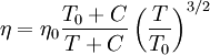
Effect of temperature on the viscosity of a gasSutherland's formula can be used to derive the dynamic viscosity of an ideal gas as a function of the temperature: where:
Valid for temperatures between 0 < T < 555 K with an error due to pressure less than 10% below 3.45 MPa Sutherland's constant and reference temperature for some gases
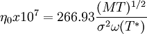
Viscosity of a dilute gasThe Chapman-Enskog equation[10] may be used to estimate viscosity for a dilute gas. This equation is based on semi-theorethical assumption by Chapman and Enskoq. The equation requires three empirically determined parameters: the collision diameter (σ), the maximum energy of attraction divided by the Boltzman constant (є/к) and the collision integral (ω(T*)).
LiquidsIn liquids, the additional forces between molecules become important. This leads to an additional contribution to the shear stress though the exact mechanics of this are still controversial.[citation needed] Thus, in liquids:
The dynamic viscosities of liquids are typically several orders of magnitude higher than dynamic viscosities of gases. Viscosity of blends of liquidsThe viscosity of the blend of two or more liquids can be estimated using the Refutas equation[11][12]. The calculation is carried out in three steps. The first step is to calculate the Viscosity Blending Number (VBN) (also called the Viscosity Blending Index) of each component of the blend:
where v is the viscosity in centistokes (cSt). It is important that the viscosity of each component of the blend be obtained at the same temperature. The next step is to calculate the VBN of the blend, using this equation:
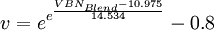
where xX is the mass fraction of each component of the blend. Once the viscosity blending number of a blend has been calculated using equation (2), the final step is to determine the viscosity of the blend by solving equation (1) for v:
where VBNBlend is the viscosity blending number of the blend. Viscosity of materialsThe viscosity of air and water are by far the two most important materials for aviation aerodynamics and shipping fluid dynamics. Temperature plays the main role in determining viscosity. Viscosity of airThe viscosity of air depends mostly on the temperature. At 15.0 °C, the viscosity of air is 1.78 × 10⁻⁵ kg/(m·s). One can get the viscosity of air as a function of temperature from the Gas Viscosity Calculator Viscosity of waterThe viscosity of water is 8.90 × 10⁻⁴ Pa·s or 8.90 × 10⁻³ dyn·s/cm2 at about 25 °C. Viscosity of various materials
Some dynamic viscosities of Newtonian fluids are listed below:
* Data from CRC Handbook of Chemistry and Physics, 73rd edition, 1992-1993. Fluids with variable compositions, such as honey, can have a wide range of viscosities. A more complete table can be found here, including the following:
* These materials are highly non-Newtonian. Viscosity of solidsOn the basis that all solids flow to a small extent in response to shear stress some researchers[14][15] have contended that substances known as amorphous solids, such as glass and many polymers, may be considered to have viscosity. This has led some to the view that solids are simply liquids with a very high viscosity, typically greater than 1012 Pa·s. This position is often adopted by supporters of the widely held misconception that glass flow can be observed in old buildings. This distortion is more likely the result of glass making process rather than the viscosity of glass.[16] However, others argue that solids are, in general, elastic for small stresses while fluids are not.[17] Even if solids flow at higher stresses, they are characterized by their low-stress behavior. Viscosity may be an appropriate characteristic for solids in a plastic regime. The situation becomes somewhat confused as the term viscosity is sometimes used for solid materials, for example Maxwell materials, to describe the relationship between stress and the rate of change of strain, rather than rate of shear. These distinctions may be largely resolved by considering the constitutive equations of the material in question, which take into account both its viscous and elastic behaviors. Materials for which both their viscosity and their elasticity are important in a particular range of deformation and deformation rate are called viscoelastic. In geology, earth materials that exhibit viscous deformation at least three times greater than their elastic deformation are sometimes called rheids. Viscosity of amorphous materials
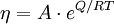
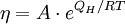
Viscous flow in amorphous materials (e.g. in glasses and melts) [19][20][21] is a thermally activated process:
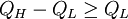
where Q is activation energy, T is temperature, R is the molar gas constant and A is approximately a constant. The viscous flow in amorphous materials is characterised by a deviation from the Arrhenius-type behaviour: Q changes from a high value QH at low temperatures (in the glassy state) to a low value QL at high temperatures (in the liquid state). Depending on this change, amorphous materials are classified as either
The fragility of amorphous materials is numerically characterized by the Doremus’ fragility ratio: RD = QH / QL and strong material have The viscosity of amorphous materials is quite exactly described by a two-exponential equation:
with constants A1,A2,B,C and D related to thermodynamic parameters of joining bonds of an amorphous material. Not very far from the glass transition temperature, Tg, this equation can be approximated by a Vogel-Tammann-Fulcher (VTF) equation or a Kohlrausch-type stretched-exponential law. If the temperature is significantly lower than the glass transition temperature,
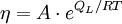
with: QH = Hd + Hm where Hd is the enthalpy of formation of broken bonds (termed configurons) and Hm is the enthalpy of their motion. When the temperature is less than the glass transition temperature, T < Tg, the activation energy of viscosity is high because the amorphous materials are in the glassy state and most of their joining bonds are intact. If the temperature is highly above the glass transition temperature,
with: QL = Hm When the temperature is higher than the glass transition temperature, T > Tg, the activation energy of viscosity is low because amorphous materials are melt and have most of their joining bonds broken which facilitates flow. Volume (Bulk) viscosityThe negative-one-third of the trace of the stress tensor is often identified with the thermodynamic pressure,
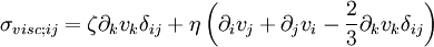
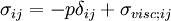
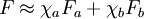
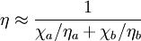
which only depends upon the equilibrium state potentials like temperature and density (equation of state). In general, the trace of the stress tensor is the sum of thermodynamic pressure contribution plus another contribution which is proportional to the divergence of the velocity field. This constant of proportionality is called the volume viscosity. Eddy viscosityIn the study of turbulence in fluids, a common practical strategy for calculation is to ignore the small-scale vortices (or eddies) in the motion and to calculate a large-scale motion with an eddy viscosity that characterizes the transport and dissipation of energy in the smaller-scale flow (see large eddy simulation). Values of eddy viscosity used in modeling ocean circulation may be from 5x10⁴ to 106 Pa·s depending upon the resolution of the numerical grid. FluidityThe reciprocal of viscosity is fluidity, usually symbolized by φ = 1 / η or F = 1 / η, depending on the convention used, measured in reciprocal poise (cm·s·g-1), sometimes called the rhe. Fluidity is seldom used in engineering practice. The concept of fluidity can be used to determine the viscosity of an ideal solution. For two components a and b, the fluidity when a and b are mixed is which is only slightly simpler than the equivalent equation in terms of viscosity: where χa and χb is the mole fraction of component a and b respectively, and ηa and ηb are the components pure viscosities. The linear viscous stress tensor(See Hooke's law and strain tensor for an analogous development for linearly elastic materials.) Viscous forces in a fluid are a function of the rate at which the fluid velocity is changing over distance. The velocity at any point where
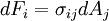
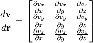
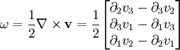
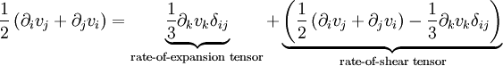
This is just the Jacobian of the velocity field. Viscous forces are the result of relative motion between elements of the fluid, and so are expressible as a function of the velocity field. In other words, the forces at If we represent x, y, and z by indices 1, 2, and 3 respectively, the i,j component of the Jacobian may be written as Any matrix may be written as the sum of an antisymmetric matrix and a symmetric matrix, and this decomposition is independent of coordinate system, and so has physical significance. The velocity field may be approximated as: where Einstein notation is now being used in which repeated indices in a product are implicitly summed. The second term from the right is the asymmetric part of the first derivative term, and it represents a rigid rotation of the fluid about For such a rigid rotation, there is no change in the relative positions of the fluid elements, and so there is no viscous force associated with this term. The remaining symmetric term is responsible for the viscous forces in the fluid. Assuming the fluid is isotropic (i.e. its properties are the same in all directions), then the most general way that the symmetric term (the rate-of-strain tensor) can be broken down in a coordinate-independent (and therefore physically real) way is as the sum of a constant tensor (the rate-of-expansion tensor) and a traceless symmetric tensor (the rate-of-shear tensor): where δij is the unit tensor. The most general linear relationship between the stress tensor where ζ is the coefficient of bulk viscosity (or "second viscosity") and η is the coefficient of (shear) viscosity. The forces in the fluid are due to the velocities of the individual molecules. The velocity of a molecule may be thought of as the sum of the fluid velocity and the thermal velocity. The viscous stress tensor described above gives the force due to the fluid velocity only. The force on an area element in the fluid due to the thermal velocities of the molecules is just the hydrostatic pressure. This pressure term ( − pδij) must be added to the viscous stress tensor to obtain the total stress tensor for the fluid. The infinitesimal force dFi on an infinitesimal area dAi is then given by the usual relationship: See also
References
Additional reading
Categories: Continuum mechanics | Viscosity |
||||||||||||||||||||||||||||||||||||||||||||||||||||||||||||||||||||||||||||||||||||||||||||||||||||||||||||||||||||||||||||||||||
| This article is licensed under the GNU Free Documentation License. It uses material from the Wikipedia article "Viscosity". A list of authors is available in Wikipedia. |


 .
.
 .
.
 ; T*=κT/ε
![\mbox{VBN} = 14.534 \times ln[ln(v + 0.8)] + 10.975\,](images/math/1/3/b/13b94da2c908803b06788fc44a57d36c.png)
![\mbox{VBN}_\mbox{Blend} = [x_A \times \mbox{VBN}_A] + [x_B \times \mbox{VBN}_B] + ... + [x_N \times \mbox{VBN}_N]\,](images/math/1/2/7/127755015f8dae0457442415bd300781.png)
 whereas fragile materials have
![\eta = A_1 \cdot T \cdot [1 + A_2 \cdot e^{B/RT}] \cdot [1 + C \cdot e^{D/RT}]](images/math/2/c/3/2c36bb3609cd14e755de5a6c44a5d96f.png)
 , then the two-exponential equation simplifies to an Arrhenius type equation:
 , the two-exponential equation also simplifies to an Arrhenius type equation:
 ,
,
 is specified by the velocity field
  . The velocity at a small distance
  from point
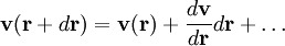
 is shorthand for the dyadic product of the del operator and the velocity:
 where
where  is shorthand for
  . Note that when the first and higher derivative terms are zero, the velocity of all fluid elements is parallel, and there are no viscous forces.

 and the rate-of-strain tensor is then a linear combination of these two tensors: