To use all functions of this page, please activate cookies in your browser.
My watch list
my.chemeurope.com
my.chemeurope.com
With an accout for my.chemeurope.com you can always see everything at a glance – and you can configure your own website and individual newsletter.
- My watch list
- My saved searches
- My saved topics
- My newsletter
Navier-Stokes equations
The Navier-Stokes equations, named after Claude-Louis Navier and George Gabriel Stokes, describe the motion of fluid substances such as liquids and gases. These equations establish that changes in momentum in infinitesimal volumes of fluid are simply the sum of dissipative viscous forces (similar to friction), changes in pressure, gravity, and other forces acting inside the fluid: an application of Newton's second law. They are one of the most useful sets of equations because they describe the physics of a large number of phenomena of academic and economic interest. They may be used to model weather, ocean currents, water flow in a pipe, flow around an airfoil (wing), and motion of stars inside a galaxy. As such, these equations in both full and simplified forms, are used in the design of aircraft and cars, the study of blood flow, the design of power stations, the analysis of the effects of pollution, etc. Coupled with Maxwell's equations they can be used to model and study magnetohydrodynamics. The Navier-Stokes equations are also of great interest in a purely mathematical sense. Somewhat surprisingly, given their wide range of practical uses, mathematicians have yet to prove that in three dimensions solutions always exist (existence), or that if they do exist they do not contain any infinities, singularities or discontinuities (smoothness). These are called the Navier-Stokes existence and smoothness problems. The Clay Mathematics Institute has called this one of the seven most important open problems in mathematics, and offered a $1,000,000 prize for a solution or a counter-example. The Navier-Stokes equations are differential equations which, unlike algebraic equations, do not explicitly establish a relation among the variables of interest (e.g. velocity and pressure). Rather, they establish relations among the rates of change. For example, the Navier-Stokes equations for simple case of an ideal fluid (inviscid) can state that acceleration (the rate of change of velocity) is proportional to the gradient (a type of multivariate derivative) of pressure. Contrary to what is normally seen in solid mechanics, the Navier-Stokes equations dictate not position but rather velocity. A solution of the Navier-Stokes equations is called a velocity field or flow field, which is a description of the velocity of the fluid at a given point in space and time. Once the velocity field is solved for, other quantities of interest (such as flow rate, drag force, or the path a "particle" of fluid will take) may be found. Product highlight
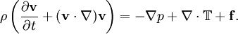
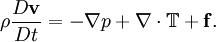
PropertiesNonlinearityThe Navier-Stokes equations are nonlinear partial differential equations in almost any real situation (an exception is creeping flow). The nonlinearity makes most problems difficult or impossible to solve and is part of the cause of turbulence. The nonlinearity is due to convective acceleration, which is an acceleration associated with the change in velocity over position. Hence, any convective flow, whether turbulent or not, will involve nonlinearity, an example of convective but laminar (nonturbulent) flow would be the passage of a viscous fluid (for example, oil) through a small converging nozzle. Such flows, whether exactly solvable or not, can often be thoroughly studied and understood. TurbulenceTurbulence is the time dependent chaotic behavior seen in many fluid flows. It is generally believed that it is due to the inertia of the fluid as a whole: the culmination of time dependent and convective acceleration; hence flows where inertial effects are small tend to be laminar (the Reynolds number quantifies how much the flow is affected by inertia). It is believed, though not known with certainty, that the Navier-Stokes equations model turbulence properly. Even though turbulence is an everyday experience, it is extremely difficult to find solutions, quantify, or in general characterize. A $1,000,000 prize was offered in May 2000 by the Clay Mathematics Institute to whoever makes preliminary progress toward a mathematical theory which will help in the understanding of this phenomenon. The numerical solution of the Navier-Stokes equations for turbulent flow is extremely difficult, and due to the significantly different mixing-length scales that are involved in turbulent flow, the stable solution of this requires such a fine mesh resolution that the computational time becomes significantly infeasible for calculation. Attempts to solve turbulent flow using a laminar solver typically result in a time-unsteady solution, which fails to converge appropriately. To counter this, several approximations such as the Reynold's averaged Navier-Stokes equations and the k-ε model are used in practical CFD applications when modelling turbulent flows. ApplicabilityTogether with supplemental equations (for example, conservation of mass) and well formulated boundary conditions, the Navier-Stokes equations seem to model fluid motion accurately; even turbulent flows seem (on average) to agree with real world observations. The Navier-Stokes equations assume that the fluid being studied is a continuum. At very small scales or under extreme conditions, real fluids made out of discrete molecules will produce results different from the continuous fluids modeled by the Navier-Stokes equations. Depending on the Knudsen number of the problem, statistical mechanics or possibly even molecular dynamics may be a more appropriate approach. Another limitation is very simply the complicated nature of the equations. Time tested formulations exist for common fluid families, but the application of the Navier-Stokes equations to less common families tends to result in very complicated formulations which are an area of current research. For this reason, the Navier-Stokes equations are usually written for Newtonian fluids. Derivation and descriptionThe derivation of the Navier-Stokes equations begins with the conservation of mass, momentum, and energy being written for an arbitrary control volume. In an inertial frame of reference, the most general form of the Navier-Stokes equations ends up being: This is a statement of the conservation of momentum in a fluid, it is an application of Newton's second law to a continuum. This equation is often written using the substantive derivative, making it more apparent that this is a statement of Newton's law: The left side of the equation describes acceleration, and may be composed of time dependent or convective effects (also the effects of non-inertial coordinates if present). The right side of the equation is in effect a summation of body forces.
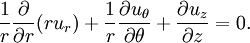
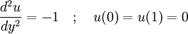
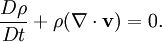
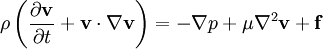
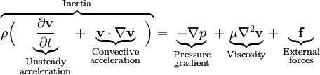
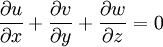
The viscous term The Navier-Stokes equations are strictly a statement of the conservation of momentum. In order to fully describe fluid flow, more information is needed (how much depends on the assumptions made), this may include the conservation of mass, the conservation of energy, or an equation of state. Regardless of the flow assumptions, a statement of the conservation of mass is nearly always necessary. This is achieved through the mass continuity equation, given in its most general form as: or, using the substantive derivative: Incompressible flow of Newtonian fluidsThe vast majority of work on the Navier-Stokes equations is done under an incompressible flow assumption for Newtonian fluids. The incompressible flow assumption typically holds well even when dealing with a "compressible" fluid, such as air at room temperature (even when flowing up to about Mach 0.3). Taking the incompressible flow assumption into account and assuming constant viscosity, the Navier-Stokes equations will read (in vector form): f represents "other" body forces (forces per unit volume), such as gravity or centrifugal force. It's well worth observing the meaning of each term: Note that only the convective terms are nonlinear for incompressible Newtonian flow. The convective acceleration is an acceleration caused by a (possibly steady) change in velocity over position, for example the speeding up of fluid entering a converging nozzle. Though individual fluid particles are being accelerated and thus are under unsteady motion, the flow field (a velocity distribution) will not necessarily be time dependent. Another important observation is that the viscosity is represented by the vector Laplacian of the velocity field. This implies that Newtonian viscosity is diffusion of momentum, this works in much the same way as the diffusion of heat seen in the heat equation (which also involves the Laplacian). If temperature effects are also neglected, the only "other" equation needed is the continuity equation. Under the incompressible assumption, density is a constant and it follows that the equation will simplify to: This is more specifically a statement of the conservation of volume (see divergence). If temperature effects are additionally assumed negligible, this is the only supplemental equation needed. These equations are commonly used in 3 coordinates systems: Cartesian, cylindrical, and spherical. The Cartesian equations follow directly from the vector equation above, obtaining equations in other coordinate systems will require a change of variables. Cartesian coordinatesWriting the vector equation explicitly, Note that gravity has been accounted for as a body force, and the values of gx,gy,gz will depend on the orientation of gravity with respect to the chosen set of coordinates. The continuity equation reads: Note that the velocity components (the dependent variables to be solved for) are u, v, w. This system of four equations compromises the most commonly used and studied form. Though comparatively more compact than other representations, this is a nonlinear system of partial differential equations for which solutions are difficult to obtain. Cylindrical coordinatesA change of variables on the Cartesian equations will yield the following momentum equations for r, θ, and z: The gravity components will generally not be constants, however for most applications either the coordinates are chosen so that the gravity components are constant or else it is assumed that gravity is counteracted by a pressure field (for example, flow in horizontal pipe is treated normally without gravity and without a vertical pressure gradient). The continuity equation is: This cylindrical representation of the incompressible Navier-Stokes equations is the second most commonly seen (the first being Cartesian above). Compressible flow of Newtonian fluidsThere are some exceptional phenomena that are closely linked with fluid compressibility. One of the obvious examples is sound. Description of such phenomena requires more general presentation of the Navier-Stokes equation that takes into account fluid compressibility. If viscosity is assumed a constant, one additional term appears, as shown here: where μv is second viscosity coefficient. It is related to volume viscosity or bulk viscosity. This additional term disappears for incompressible fluid, when the divergence of the flow equals 0. Application to specific problemsThe Navier-Stokes equations, even when written explicitly for specific fluids, are rather generic in nature and their proper application to specific problems can be very diverse. This is partly because there is an enormous variety of problems that may be modeled, ranging from as simple as the distribution of static pressure to as complicated as multiphase flow driven by surface tension. Generally, application to specific problems begins with some flow assumptions and initial/boundary condition formulation, this may be followed by scale analysis to further simplify the problem. For example, after assuming steady, parallel, one dimensional, nonconvective pressure driven flow between parallel plates, the resulting scaled (dimensionless) boundary value problem is:
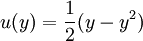
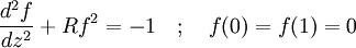
The boundary condition is the no slip condition. This problem is easily solved for the flow field: From this point onward more quantities of interest can be easily obtained, such as viscous drag force or net flow rate. Difficulties may arise when the problem becomes slightly more complicated. A seemingly modest twist on the parallel flow above would be the radial flow between parallel plates; this involves convection and thus nonlinearity. The velocity field may be represented by a function f(z) that must satisfy: This ordinary differential equation is what is obtained when the Navier-Stokes equations are written and the flow assumptions applied (additionally, the pressure gradient is solved for). The nonlinear term makes this a very difficult problem to solve analytically (a lengthy implicit solution may be found which involves elliptic integrals and roots of cubic polynomials). Issues with the actual existence of solutions arise for R > 22.609 (approximately), the parameter R being similar to the Reynolds number. This is an example of flow assumptions losing their applicability, and an example of the difficulty in "high" Reynolds number flows. See also
References
Categories: Continuum mechanics | Equations of fluid dynamics |
|||||||||||||
| This article is licensed under the GNU Free Documentation License. It uses material from the Wikipedia article "Navier-Stokes_equations". A list of authors is available in Wikipedia. |


 and
and  are gradients of surface forces and represent stresses inside the fluid, analogous to stresses in a solid.
  represents "other" forces, such as gravity.
 when the fluid is assumed incompressible and
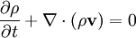


![\rho \left(\frac{\partial u_r}{\partial t} + u_r \frac{\partial u_r}{\partial r} + \frac{u_{\theta}}{r} \frac{\partial u_r}{\partial \theta} + u_z \frac{\partial u_r}{\partial z} - \frac{u_{\theta}^2}{r}\right) = -\frac{\partial p}{\partial r} + \mu \left[\frac{\partial}{\partial r}\frac{1}{r}\left( \frac{\partial ru_r}{\partial r}\right) + \frac{1}{r^2}\frac{\partial^2 u_r}{\partial \theta^2} + \frac{\partial^2 u_r}{\partial z^2} - \frac{2}{r^2}\frac{\partial u_{\theta}}{\partial \theta}\right] + \rho g_r](images/math/6/d/1/6d102be9ff6690c863d2dab1fccf8c91.png)
![\rho \left(\frac{\partial u_{\theta}}{\partial t} + u_r \frac{\partial u_{\theta}}{\partial r} + \frac{u_{\theta}}{r} \frac{\partial u_{\theta}}{\partial \theta} + u_z \frac{\partial u_{\theta}}{\partial z} + \frac{u_r u_{\theta}}{r}\right) = -\frac{1}{r}\frac{\partial p}{\partial \theta} + \mu \left[\frac{\partial}{\partial r}\frac{1}{r}\left( \frac{\partial ru_{\theta}}{\partial r}\right) + \frac{1}{r^2}\frac{\partial^2 u_{\theta}}{\partial \theta^2} + \frac{\partial^2 u_{\theta}}{\partial z^2} + \frac{2}{r^2}\frac{\partial u_r}{\partial \theta} \right] + \rho g_{\theta}](images/math/d/2/a/d2a964526a5644387c6d2f6a080f0039.png)
![\rho \left(\frac{\partial u_z}{\partial t} + u_r \frac{\partial u_z}{\partial r} + \frac{u_{\theta}}{r} \frac{\partial u_z}{\partial \theta} + u_z \frac{\partial u_z}{\partial z}\right) = -\frac{\partial p}{\partial z} + \mu \left[\frac{\partial}{\partial r}\frac{1}{r}\left( \frac{\partial ru_z}{\partial r}\right) + \frac{1}{r^2}\frac{\partial^2 u_z}{\partial \theta^2} + \frac{\partial^2 u_z}{\partial z^2}\right] + \rho g_z](images/math/8/6/e/86e9d6a95aeb7193f553bb7be0509dc8.png)