To use all functions of this page, please activate cookies in your browser.
My watch list
my.chemeurope.com
my.chemeurope.com
With an accout for my.chemeurope.com you can always see everything at a glance – and you can configure your own website and individual newsletter.
- My watch list
- My saved searches
- My saved topics
- My newsletter
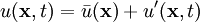
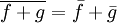
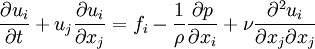
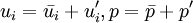
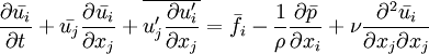
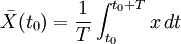
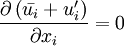
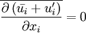
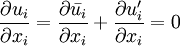
Reynolds-averaged Navier-Stokes equationsThe Reynolds-averaged Navier-Stokes (RANS) equations are time-averaged [1] equations of motion for fluid flow. They are primarily used while dealing with turbulent flows. These equations can be used with approximations based on knowledge of the properties of flow turbulence to give approximate averaged solutions to the Navier-Stokes equations. For an incompressible flow of Newtonian fluid, these equations can be written as Product highlightThe left hand side of this equation represents the change in mean momentum of fluid element due to the unsteadiness in the mean flow and the convection by the mean flow. This change is balanced by the mean body force, the isotropic stress due to the mean pressure field, the viscous stresses, and apparent stress Derivation of RANS equationsThe basic tool required for the derivation of the RANS equations from the instantaneous Navier-Stokes equations is the Reynolds decomposition. Reynolds decomposition refers to separation of the flow variable (like velocity u) into the mean (time-averaged) component ( where, The following rules will be useful while deriving the RANS. If f and g are two flow variables (like density (ρ), velocity (u), pressure (p), etc.) and s is one of the independent variables (x,y,z, or t) then, Now the Navier-Stokes equations of motion [4] for an incompressible Newtonian fluid are: Substituting,
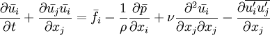
The momentum equation can also be written as, [6] On further manipulations this yields, where,
Notes
Categories: Equations of fluid dynamics | Turbulence models |
| This article is licensed under the GNU Free Documentation License. It uses material from the Wikipedia article "Reynolds-averaged_Navier-Stokes_equations". A list of authors is available in Wikipedia. |
![\rho \frac{\partial \bar{u}_i}{\partial t} + \rho \frac{\partial \bar{u}_j \bar{u}_i }{\partial x_j} = \rho \bar{f}_i + \frac{\partial}{\partial x_j} \left[ - \bar{p}\delta_{ij} + \mu \left( \frac{\partial \bar{u}_i}{\partial x_j} + \frac{\partial \bar{u}_j}{\partial x_i} \right) - \rho \overline{u_i^\prime u_j^\prime} \right ].](images/math/3/b/6/3b6c7cc07bead7a5f14f643286616b1b.png)


 due to the fluctuating velocity field, generally referred to as
  ) and the fluctuating component (
 ).
).
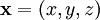 is the position vector.


 , etc.
![\rho \frac{\partial \bar{u_i}}{\partial t} + \rho \frac{\partial \bar{u_j} \bar{u_i} }{\partial x_j} = \rho \bar{f_i} + \frac{\partial}{\partial x_j} \left[ - \bar{p}\delta_{ij} + 2\mu \bar{S_{ij}} - \rho \overline{u_i^\prime u_j^\prime} \right ]](images/math/3/a/6/3a62f01591e2d0a13082bc779c54e5a6.png)
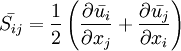 is the mean rate of strain of strain tensor.
 ) of a variable (
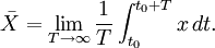
 ).
).  to represent the instantaneous, mean and fluctuating term.


 ) can be simplified to,

Last viewed


