To use all functions of this page, please activate cookies in your browser.
My watch list
my.chemeurope.com
my.chemeurope.com
With an accout for my.chemeurope.com you can always see everything at a glance – and you can configure your own website and individual newsletter.
- My watch list
- My saved searches
- My saved topics
- My newsletter
Heat equationThe heat equation is an important partial differential equation which describes the variation of temperature in a given region over time. Product highlight
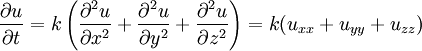
General-audience descriptionSuppose one has a function u which describes the temperature at a given location (x, y, z). This function will change over time as heat spreads throughout space. The heat equation is used to determine the change in the function u over time. The image below is animated and has a description of the way heat changes in time along a metal bar. One of the interesting properties of the heat equation is the maximum principle which says that the maximum value of u is either earlier in time than the region of concern or on the edge of the region of concern. This is essentially saying that temperature comes either from some source or from earlier in time because heat permeates but is not created from nothingness. This is a property of parabolic partial differential equations and is not difficult to prove mathematically (see below). Another interesting property is that even if u has a discontinuity at an initial time t = t0, then the temperature becomes instantly smooth as soon as t > t0. For example, if a bar of metal has temperature 0 and another has temperature 100 and they are stuck together end to end, then instantaneously the temperature at the point of connection is 50 and the graph of the temperature is smoothly running from 0 to 100. This is not physically possible, since there would then be information propagation at infinite speed, which would violate causality. Therefore this is a property of the mathematical equation rather than of heat conduction itself. However, for most practical purposes, the difference is negligible. The heat equation is used in probability and describes random walks. It is also applied in financial mathematics for this reason. It is also important in Riemannian geometry and thus topology: it was adapted by Richard Hamilton when he defined the Ricci flow that was later used to solve the topological Poincaré conjecture. See also the Dirac delta function. The physical problem and the equationIn the special case of heat propagation in an isotropic and homogeneous medium in the 3-dimensional space, this equation is where:
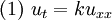
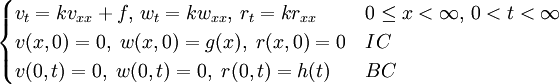
The heat equation is a consequence of Fourier's law of cooling (see heat conduction). If the medium is not the whole space, in order to solve the heat equation uniquely we also need to specify boundary conditions for u. To determine uniqueness of solutions in the whole space it is necessary to assume an exponential bound on the growth of solutions, this assumption is consistent with observed experiments. Solutions of the heat equation are characterized by a gradual smoothing of the initial temperature distribution by the flow of heat from warmer to colder areas of an object. Generally, many different states and starting conditions will tend toward the same stable equilibrium. As a consequence, to reverse the solution and conclude something about earlier times or initial conditions from the present heat distribution is very inaccurate except over the shortest of time periods. The heat equation is the prototypical example of a parabolic partial differential equation. Using the Laplace operator, the heat equation can be simplified, and generalized to similar equations over spaces of arbitrary number of dimensions, as where the Laplace operator, Δ or The heat equation governs heat diffusion, as well as other diffusive processes, such as particle diffusion or the propagation of action potential in nerve cells. Although they are not diffusive in nature, some quantum mechanics problems are also governed by a mathematical analog of the heat equation (see below). It also can be used to model some phenomena arising in finance, like the Black-Scholes or the Ornstein-Uhlenbeck processes. The equation, and various non-linear analogues, has also been used in image analysis. The heat equation is, technically, in violation of special relativity, because its solutions involve instantaneous propagation of a disturbance. The part of the disturbance outside the forward light cone can usually be safely neglected, but if it is necessary to develop a reasonable speed for the transmission of heat, a hyperbolic problem should be considered instead -- like a partial differential equation involving a second-order time derivative. Solving the heat equation using Fourier seriesThe following solution technique for the heat equation was proposed by Joseph Fourier in his treatise Théorie analytique de la chaleur, published in 1822. Let us consider the heat equation for one space variable. This could be used to model heat conduction in a rod. The equation is where u = u(t, x) is a function of two variables t and x. Here
We assume the initial condition where the function f is given and the boundary conditions
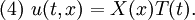
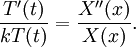
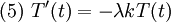
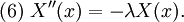
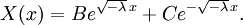
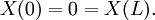
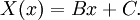
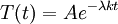
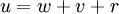
Let us attempt to find a solution of (1) which is not identically zero satisfying the boundary conditions (3) but with the following property: u is a product in which the dependence of u on x, t is separated, that is: This solution technique is called separation of variables. Substituting u back into equation (1), Since the right hand side depends only on x and the left hand side only on t, both sides are equal to some constant value − λ. Thus: and We will now show that solutions for (6) for values of λ ≤ 0 cannot occur:
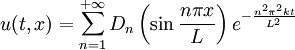
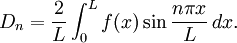
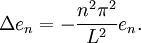
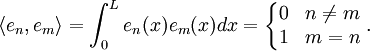
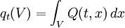
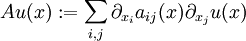
This solves the heat equation in the special case that the dependence of u has the special form (4). In general, the sum of solutions to (1) which satisfy the boundary conditions (3) also satisfies (1) and (3). We can show that the solution to (1), (2) and (3) is given by where Generalizing the solution techniqueThe solution technique used above can be greatly extended to many other types of equations. The idea is that the operator uxx with the zero boundary conditions can be represented in terms of its eigenvectors. This leads naturally to one of the basic ideas of the spectral theory of linear self-adjoint operators. Consider the linear operator Δ u = ux x. The infinite sequence of functions for n ≥ 1 are eigenvectors of Δ. Indeed Moreover, any eigenvector f of Δ with the boundary conditions f(0)=f(L)=0 is of the form en for some n ≥ 1. The functions en for n ≥ 1 form an orthonormal sequence with respect to a certain inner product on the space of real-valued functions on [0, L]. This means Finally, the sequence {en}n ∈ N spans a dense linear subspace of L2(0, L). This shows that in effect we have diagonalized the operator Δ. Heat conduction in non-homogeneous anisotropic mediaIn general, the study of heat conduction is based on several principles. Heat flow is a form of energy flow, and as such it is meaningful to speak of the time rate of flow of heat into a region of space.
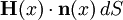
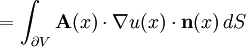
Thus the rate of heat flow into V is also given by the surface integral where n(x) is the outward pointing normal vector at x.
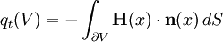
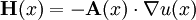
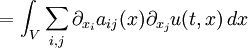
By Green's theorem, the previous surface integral for heat flow into V can be transformed into the volume integral
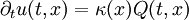
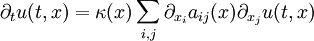
Putting these equations together gives the general equation of heat flow: Remarks.
is self-adjoint and dissipative, thus by the spectral theorem it generates a one-parameter semigroup. Particle diffusionParticle diffusion equationOne can model particle diffusion by an equation involving either:
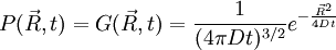
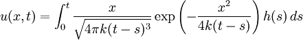
In either case, one uses the heat equation or Both c and P are functions of position and time. D is the diffusion coefficient that controls the speed of the diffusive process, and is typically expressed in meters squared over second. If the diffusion coefficient D is not constant, but depends on the concentration c (or P in the second case), then one gets the nonlinear diffusion equation. The random trajectory of a single particle subject to the particle diffusion equation is a brownian motion. If a particle is placed in It is related to the probability density functions associated to each of its components Rx, Ry and Rz in the following way: The random variables Rx, Ry and Rz are distributed according to a normal distribution of mean 0 and of variance At t=0, the expression of Historical origin of the diffusion equationThe particle diffusion equation was originally derived by Adolf Fick in 1855. Solving the diffusion equation through Green functionsGreen functions are the solutions of the diffusion equation corresponding to the initial condition of a particle of known position. For another initial condition, the solution to the diffusion equation can be expressed as a decomposition on a set of Green Functions. Say, for example, that at t=0 we have not only a particle located in a known position As any function, the initial concentration profile can be decomposed as an integral sum on Dirac delta functions: At subsequent instants, given the linearity of the diffusion equation, the concentration profile becomes:
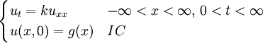
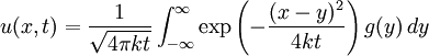
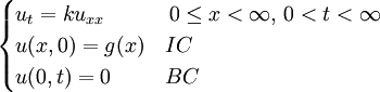
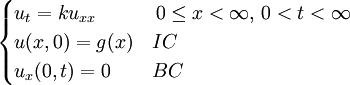
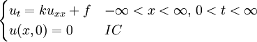
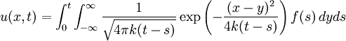
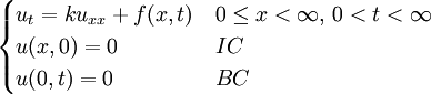
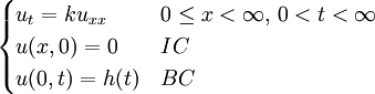
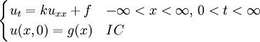
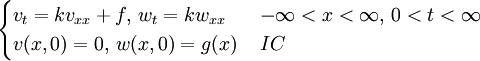
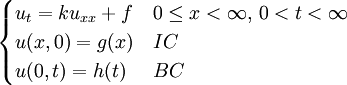
Although it is more easily understood in the case of particle diffusion , where an initial condition corresponding to a Dirac delta function can be intuitively described as a particle being located in a known position, such a decomposition of a solution into Green functions can be generalized to the case of any diffusive process, like heat transfer, or momentum diffusion, which is the phenomenon at the origin of viscosity in liquids. List of Green function solutions in 1D
Schrödinger equation for a free particleWith a simple division, the Schrödinger equation for a single particle of mass m in the absence of any applied force field can be rewritten in the following way:
This equation is a mathematical analogue of the particle diffusion equation, which one obtains through the following transformation: Applying this transformation to the expressions of the Green functions determined in the case of particle diffusion yields the Green functions of the Schrödinger equation, which in turn can be used to obtain the wavefunction at any time through an integral on the wavefunction at t=0:
Diffusion (of particles, heat, momentum...) describes the return to global thermodynamic equilibrium of an inhomogeneous system, and as such is a time-irreversible phenomenon, associated to an increase in the entropy of the universe: in the case of particle diffusion, if As a generalization of classical mechanics, quantum mechanics involves only time-reversible phenomena: if It is the imaginary nature of the equivalent diffusion coefficient On a related note, it is interesting to notice that the imaginary exponentials that appear in the Green functions associated to the Schrödinger equation create interferences between the various components of the decomposition of the wavefunction. This is a symptom of the wavelike properties of quantum particles. ApplicationsThe heat equation arises in the modeling of a number of phenomena and is often used in financial mathematics in the modeling of options. The famous Black-Scholes option pricing model's differential equation can be transformed into the heat equation allowing relatively easy solutions from a familiar body of mathematics. Many of the extensions to the simple option models do not have closed form solutions and thus must be solved numerically to obtain a modeled option price. The heat equation can be efficiently solved numerically using the Crank-Nicolson method and this method can be extended to many of the models with no closed form solution. (Wilmott, 1995) An abstract form of heat equation on manifolds provides a major approach to the Atiyah-Singer index theorem, and has led to much further work on heat equations in Riemannian geometry. See also
References
Categories: Heat conduction | Diffusion |
|
| This article is licensed under the GNU Free Documentation License. It uses material from the Wikipedia article "Heat_equation". A list of authors is available in Wikipedia. |


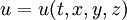 is temperature as a function of time and space;
 is the rate of change of temperature at a point over time;
 ,
,  , and
, and  are the second spatial derivatives (thermal conductions) of temperature in the x, y, and z directions, respectively
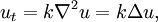
 , the divergence of the gradient, is taken in the spatial variables.
![(2) \ u(0,x) = f(x) \quad \forall x \in [0,L] \quad](images/math/c/a/5/ca5655ee90542959d5fa15ca07ff36e0.png)
 .
.


 at time
  will be the following:

 . In 3D, the random vector
  and of variance
  .
.
 above is singular. The probability density function corresponding to the initial condition of a particle located in a known position
  (the generalisation to 3D of the Dirac delta function is simply
 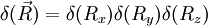 ). The solution of the diffusion equation associated to this initial condition is also called a Green function.
 . Solving the diffusion equation will tell us how this profile will evolve with time.

 , where
  is the Green function defined above.


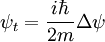 , where i is the unit imaginary number, and
  is Planck's constant divided by
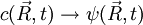

 , with
 is a solution of the diffusion equation, then
  isn't. Intuitively we know that particle diffusion tends to resorb spatial concentration inhomogeneities, and never amplify them.
 is a solution of the Schrödinger equation, then the complex conjugate of
  is also a solution. Note that the complex conjugate of a wavefunction has the exact same physical meaning as the wavefunction itself: the two react exactly in the same way to any series of quantum measurements.
 that makes up for this difference in behavior between quantum and diffusive systems.
Last viewed


