To use all functions of this page, please activate cookies in your browser.
My watch list
my.chemeurope.com
my.chemeurope.com
With an accout for my.chemeurope.com you can always see everything at a glance – and you can configure your own website and individual newsletter.
- My watch list
- My saved searches
- My saved topics
- My newsletter
Box-Muller transformA Box-Muller transform (by George Edward Pelham Box and Mervin Edgar Muller 1958)[1] is a method of generating pairs of independent standard normally distributed (zero expectation, unit variance) random numbers, given a source of uniformly distributed random numbers. It is commonly expressed in two forms. The basic form as given by Box and Muller takes two samples from the uniform distribution on the interval (0, 1] and maps them to two normally distributed samples. The polar form takes two samples from a different interval, [−1, +1], and maps them to two normally distributed samples without the use of sine or cosine functions. One could use the inverse transform sampling method to generate normally-distributed random numbers instead; the Box-Muller transform was developed to be more computationally efficient.[2] The more efficient Ziggurat algorithm can also be used. Product highlight
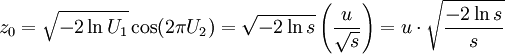
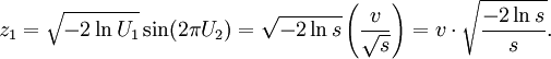
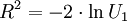
Basic formSuppose U1 and U2 are independent random variables that are uniformly distributed in the interval (0, 1]. Let and Then Z0 and Z1 are independent random variables with a normal distribution of standard deviation 1. The derivation[3] is based on the fact that, in a two-dimensional cartesian system where X and Y coordinates are described by two independent and normally distributed random variables, the random variables for R2 and Θ (shown above) in the corresponding polar coordinates are also independent and can be expressed as and Polar formThe polar form is attributed by Devroye[4] to Marsaglia. It is also mentioned without attribution in Carter.[5] Given u and v, independent and uniformly distributed in the closed interval [−1, +1], set s = R2 = u2 + v2. (Clearly We now identify the value of s with that of U1 and Just as the basic form produces two standard normal deviates, so does this alternate calculation. and Contrasting the two formsThe polar method differs from the basic method in that it is a type of rejection sampling. It throws away some generated random numbers, but it is typically faster than the basic method because it is simpler to compute (provided that the random number generator is relatively fast) and is more numerically robust.[5] It avoids the use of trigonometric functions, which are comparatively expensive in many computing environments. It throws away 1 − π/4 ≈ 21.46% of the total input uniformly distributed random number pairs generated, i.e. throws away 4/π − 1 ≈ 27.32% uniformly distributed random number pairs per Gaussian random number pair generated, requiring 4/π ≈ 1.2732 input random numbers per output random number. The basic form requires three multiplications, one logarithm, one square root, and one trigonometric function for each normal variate.[6] The polar form requires two multiplications, one logarithm, one square root, and one division for each normal variate. The effect is to replace one multiplication and one trigonometric function with a single division. See also
References
|
|
| This article is licensed under the GNU Free Documentation License. It uses material from the Wikipedia article "Box-Muller_transform". A list of authors is available in Wikipedia. |


 .) If s = 0 or s > 1, throw u and v away and try another pair (u, v). Continue until a pair with s in the open interval (0, 1) is found. Because u and v are uniformly distributed and because only points within the unit circle have been admitted, the values of s will be uniformly distributed in the open interval (0, 1), too. The latter can easily be seen by calculating the cumulative distribution function for s in the interval (0, 1). This is nothing more than the area of a circle with radius
  divided by
  . From this we find the probability density function to have the constant value 1 on the interval (0, 1). Equally so, the angle θ divided by
  is clearly uniformly distributed in the open interval (0, 1) and independent of s.
 with that of U2 in the basic form. As shown in the figure, the values of
  and
and  in the basic form can be replaced with the ratios
 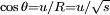 and
and  , respectively. The advantage is that calculating the trigonometric functions directly can be avoided. This is helpful when they are comparatively more expensive than the single division that replaces each one.