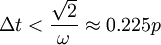
Energy drift

In molecular dynamics simulations, energy drift is the gradual change in the total energy of a closed system. According to the laws of mechanics, the energy should be a constant of motion and should not change. However, the energy does fluctuate on a short time scale and increase on a very long time scale due to numerical integration artifacts that arise with the use of a finite time step Δt. More specifically, the energy tends to increase exponentially; its increase can be understood intuitively because each step introduces a small perturbation δv to the true velocity v_true, which (if uncorrelated with v) results in a second-order increase in the energy

Additional recommended knowledge

Daily Visual Balance Check

How to quickly check pipettes?

Essential Laboratory Skills Guide

(The cross term in v · δv is zero because of no correlation.)

Energy drift - usually damping - is substantial for numerical integration schemes that are not symplectic, such as the Runge-Kutta family. Symplectic integrators usually used in molecular dynamics, such as the Verlet integrator family, exhibit increases in energy over very long time scales, though the error remains roughly constant. These integrators do not in fact reproduce the actual Hamiltonian of the system; instead, they reproduce a closely related "shadow" Hamiltonian whose value they conserve many orders of magnitude more closely. The accuracy of the energy conservation for the true Hamiltonian is dependent on the time step.^[1][2] The energy computed from the modified Hamiltonian of a symplectic integrator is from the true Hamiltonian.

Energy drift is similar to parametric resonance in that a finite, discrete timestepping scheme will result in nonphysical, limited sampling of motions with frequencies close to the frequency of velocity updates. Thus the restriction on the maximum step size that will be stable for a given system is proportional to the period of the fastest fundamental modes of the system's motion. For a motion with a natural frequency ω, artificial resonances are introduced when the frequency of velocity updates, is related to ω as

where n and m are integers describing the resonance order. For Verlet integration, resonances up to the fourth order frequently lead to numerical instability, leading to a restriction on the timestep size of

where ω is the frequency of the fastest motion in the system and p is its period.^[3] The fastest motions in most biomolecular systems involve the motions of hydrogen atoms; it is thus common to use constraint algorithms to restrict hydrogen motion and thus increase the maximum stable time step that can be used in the simulation. However, because the time scales of heavy-atom motions are not widely divergent from those of hydrogen motions, in practice this allows only about a twofold increase in time step. Common practice in all-atom biomolecular simulation is to use a time step of 1 femtosecond (fs) for unconstrained simulations and 2 fs for constrained simulations, although larger time steps may be possible for certain systems or choices of parameters.

Energy drift can also result from imperfections in evaluating the energy function, usually due to simulation parameters that sacrifice accuracy for computational speed. For example, cutoff schemes for evaluating the electrostatic forces introduce systematic errors in the energy with each time step as particles move back and forth across the cutoff radius if sufficient smoothing is not used. Particle mesh Ewald summation is one solution for this effect, but introduces artifacts of its own. Errors in the system being simulated can also induce energy drifts characterized as "explosive" that are not artifacts, but are reflective of the instability of the initial conditions; this may occur when the system has not been subjected to sufficient structural minimization before beginning production dynamics. In practice, energy drift may be measured as a percent increase over time, or as a time needed to add a given amount of energy to the system. The practical effects of energy drift depend on the simulation conditions, the thermodynamic ensemble being simulated, and the intended use of the simulation under study; for example, energy drift has much more severe consequences for simulations of the microcanonical ensemble than the canonical ensemble where the temperature is held constant. Energy drift is often used as a measure of the quality of the simulation, and has been proposed as one quality metric to be routinely reported in a mass repository of molecular dynamics trajectory data analogous to the Protein Data Bank.^[4]

References

1. ^ Gans J, Shalloway D. (2000). Shadow mass and the relationship between velocity and momentum in symplectic numerical integration. Phys. Rev. E 61(4):4587–4592.
2. ^ Engle RD, Skeel RD, Drees M. (2005). Monitoring energy drift with shadow Hamiltonians. J Comp Phys 206:432–452
3. ^ Schlick T. (2002). Molecular Modeling and Simulation: An Interdisciplinary Guide. Interdisciplinary Applied Mathematics series, vol. 21. Springer: New York, NY, USA. ISBN 0-387-95404-X. See pp420-430 for complete derivation.
4. ^ Murdock SE, Tai K, Ng MH, Johnston S, Wu B, Fangohr H, Laughton CA, Essex JW, Sansom MSP. (2006). Quality assurance for biomolecular simulations. J Chem Theory Comput 2(6): 1477-1481.

Further reading

• Sanz-Serna JM, Calvo MP. (1994). Numerical Hamiltonian Problems. Chapman & Hall, London, England.