To use all functions of this page, please activate cookies in your browser.
My watch list
my.chemeurope.com
my.chemeurope.com
With an accout for my.chemeurope.com you can always see everything at a glance – and you can configure your own website and individual newsletter.
- My watch list
- My saved searches
- My saved topics
- My newsletter
Canonical ensemble
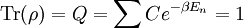
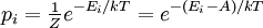
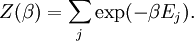
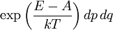
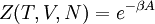
A canonical ensemble in statistical mechanics is a statistical ensemble representing a probability distribution of microscopic states of the system. The probability distribution is characterised by the proportion pi of members of the ensemble which exhibit a measurable macroscopic state i, where the proportion of microscopic states for each macroscopic state i is given by the Boltzmann distribution, where Ei is the energy of state i. It can be shown that this is the distribution which is most likely, if each system in the ensemble can exchange energy with a heat bath, or alternatively with a large number of similar systems. Equivalently, it is the distribution which has maximum entropy for a given average energy <Ei>. It is also referred to as an NVT ensemble: the number of particles (N), the volume (V), of each system in the ensemble are the same, and the ensemble has a well defined temperature (T), given by the temperature of the heat bath with which it would be in equilibrium. The quantity k is Boltzmann's constant, which relates the units of temperature to units of energy. It may be suppressed by expressing the absolute temperature using thermodynamic beta, β = 1/kT. The quantities A and Z are constants for a particular ensemble, which ensure that Σ pi is normalised to 1. Z is therefore given by
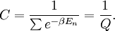
This is called the partition function of the canonical ensemble. Specifying this dependence of Z on the energies Ei conveys the same mathematical information as specifying the form of pi above. The canonical ensemble (and its partition function) is widely used as a tool to calculate thermodynamic quantites of a system under a fixed temperature. This article derives some basic elements of the canonical ensemble. Other related thermodynamic formulas are given in the partition function article. Mathematical treatments are given in the articles on the Potts model, where the canonical ensemble as a probability measure is expressed in the language of measure theory, and quantum statistical mechanics.
Product highlight
Deriving the Boltzmann factor from ensemble theoryLet Since systems in the ensemble are indistinguishable, for each set So for a given The most probable distribution is the one that maximizes
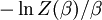
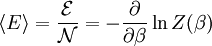
This distribution is called the canonical distribution. To determine Comparing with thermodynamic formulae, it can be shown that is identified as the Helmholtz free energy F. Consequently, from the partition function we can obtain the average thermodynamic quantities for the ensemble. For example, the average energy among members of the ensemble is
This relation can be used to determine
A derivation from heat-bath viewpointDefine the following:
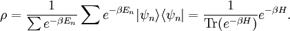
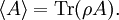
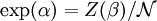
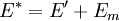
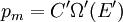
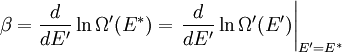
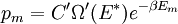
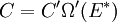
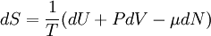
It is assumed that the system S and the reservoir S′ are in thermal equilibrium. The objective is to calculate the set of probabilities pm that S is in a particular energy state Em. Suppose S is in a microstate indexed by m. From the above definitions, the total energy of the system S* is given by Notice E* is constant, since the combined system S* is taken to be isolated. Now, arguably the key step in the derivation is that the probability of S being in the m-th state, for some constant Since Em is small compared to E*, a Taylor series expansion can be performed on the latter logarithm around the energy E*. A good approximation can be obtained by keeping the first two terms of the Taylor series expansion: The following quantity is a constant which is traditionally denoted by β, known as the thermodynamic beta. Finally, Exponentiating this expression gives The factor in front of the exponential can be treated as a normalization constant C, where From this Normalization to recover the partition functionSince probabilities must sum to 1, it must be the case that where Z is known as the partition function for the canonical ensemble. Note on derivationAs mentioned above, the derivation hinges on recognizing that the probability of the system being in a particular state is proportional to the corresponding multiplicities of the reservoir (the same can be said for the grand canonical ensemble). As long as one makes that observation, it is flexible as how one might proceed. In the derivation given, the logarithm is taken, then a linear approximation based on physical arguments is used. Alternatively, one can apply the thermodynamic identity for differential entropy: and obtain the same result. See the article on Maxwell-Boltzmann statistics where this approach is employed. The canonical ensemble is also called the Gibbs ensemble, in honor of J.W. Gibbs, widely regarded with Boltzmann as being one of the two fathers of statistical mechanics. In his definitive original book "Elementary Principles in Statistical Mechanics", Gibbs viewed an ensemble as a list of the allowed states of the system (each state appearing once and only once in the list) and the associated statistical weights. The states do not interact with each other, or with a reservoir, until Gibbs treats what happens when two complete ensembles at two different temperatures are allowed to interact weakly (Gibbs, pp 160). Gibbs writes that "...the distribution in phase..." (the phase space density in modern language) "...[is] called canonical...[if] the index of probability" (the logarithm of the statistical weight of the phase space density) "...is a linear function of the energy..." (Gibbs, Ch. 4). In Gibbs' formulation, this requirement (his equation 91, in modern notation is taken to define the canonical ensemble and to be the fundamental postulate. Gibbs does show that a large collection of interacting microcanonical systems approaches the canonical ensemble, but this is part of his demonstration (Gibbs, pp 169-183) that the principle of equal a priori probabilities, therefore the microcanonical ensemble, are inferior to the canonical ensemble as an axiomatization of statistical mechanics, at every point where the two treatments differ. Gibbs original formulation is still standard in modern mathematically rigorous treatments of statistical mechanics, where the canonical ensemble is defined as the probability measure with p and q being the canonical coordinates. Characteristic state functionThe characteristic state function of the canonical ensemble is the Helmholtz free energy function, as the following relationship holds: Quantum mechanical systemsBy applying the canonical partition function, one can easily obtain the corresponding results for a canonical ensemble of quantum mechanical systems. A quantum mechanical ensemble in general is described by a density matrix. Suppose the Hamiltonian H of interest is a self adjoint operator with only discrete spectrum. The energy levels {En} are then the eigenvalues of H, corresponding to eigenvector (Technical note: a density matrix must be trace-class, therefore we have also assumed that the sequence of energy eigenvalues diverges sufficiently fast.) A density operator is assumed to have trace 1, so , which means Q is the quantum-mechanical version of the canonical partition function. Putting C back into the eqation for ρ gives By the assumption that the energy eigenvalues diverge, the Hamiltonian H is an unbounded operator, therefore we have invoked the Borel functional calculus to exponentiate the Hamiltonian H. Alternatively, in non-rigorous fashion, one can consider that to be the exponential power series. Notice the quantity is the quantum mechanical counterpart of the canonical partition function, being the normalization factor for the mixed state of interest. The density operator ρ obtained above therefore describes the (mixed) state of a canonical ensemble of quantum mechanical systems. As with any density operator, if A is a physical observable, then its expected value is
Relations with other ensemblesA generalization of this is the grand canonical ensemble, in which the systems may share particles as well as energy. By contrast, in the microcanonical ensemble, the energy of each individual system is fixed. |
||||||||
| This article is licensed under the GNU Free Documentation License. It uses material from the Wikipedia article "Canonical_ensemble". A list of authors is available in Wikipedia. |
 .
.


 be the energy of the
  and suppose there are
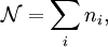
  members of the ensemble residing in this state. Further we assume the total number of systems in the ensemble,
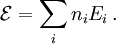
  , and the total energy of all systems of the ensemble,
  , are fixed, i.e.,
 , the number of ways of shuffling systems is equal to
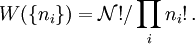
 rearrangements that specify the same state of the ensemble.
 .
To determine this distribution, one should maximize
.
To determine this distribution, one should maximize  and
and  . (The assumption that
 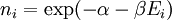 .
.
 as,
as,  . Moreover the expression
 .
.
 .
.
 , is proportional to the corresponding number of microstates available to the reservoir when S is in the m-th state. Therefore,
 . Taking the logarithm gives


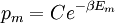


 . From the same considerations as in the classical case, the probability that a system from the ensemble will be in state
 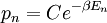 , for some constant