To use all functions of this page, please activate cookies in your browser.
My watch list
my.chemeurope.com
my.chemeurope.com
With an accout for my.chemeurope.com you can always see everything at a glance – and you can configure your own website and individual newsletter.
- My watch list
- My saved searches
- My saved topics
- My newsletter
Ensemble Kalman filter
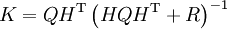
The ensemble Kalman filter (EnKF) is a recursive filter suitable for problems with a large number of variables, such as discretizations of partial differential equations in geophysical models. The EnKF originated as a version of the Kalman filter for large problems (essentially, the covariance matrix is replaced by the sample covariance), and it is now an important data assimilation component of ensemble forecasting. EnKF is related to the particle filter (in this context, a particle is the same thing as ensemble member) but the EnKF makes the assumption that all probability distributions involved are Gaussian; when it is applicable, it is much more efficient than the particle filter. This article briefly describes the derivation and practical implementation of the basic version of EnKF, and reviews several extensions.
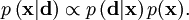
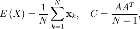
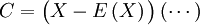
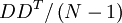
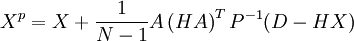
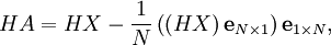
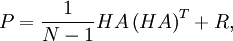
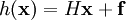
IntroductionThe Ensemble Kalman Filter (EnKF) is a Monte-Carlo implementation of the Bayesian update problem: Given a probability density function (pdf) of the state of the modeled system (the prior, called often the forecast in geosciences) and the data likelihood, the Bayes theorem is used to to obtain the pdf after the data likelihood has been taken into account (the posterior, often called the analysis). This is called a Bayesian update. The Bayesian update is combined with advancing the model in time, incorporating new data from time to time. The original Kalman Filter[1] assumes that all pdfs are Gaussian (the Gaussian assumption) and provides algebraic formulas for the change of the mean and the covariance matrix by the Bayesian update, as well as a formula for advancing the covariance matrix in time provided the system is linear. However, maintaining the covariance matrix is not feasible computationally for high-dimensional systems. For this reason, EnKFs were developed.[2][3] EnKFs represent the distribution of the system state using a collection of state vectors, called an ensemble, and replace the covariance matrix by the sample covariance computed from the ensemble. The ensemble is operated with as if it were a random sample, but the ensemble members are really not independent - the EnKF ties them together. One advantage of EnKFs is that advancing the pdf in time is achieved by simply advancing each member of the ensemble. For a survey of EnKF and related data assimilation techniques, see.[4] A version of this article is also available as the technical report.[5] A derivation of the EnKFThe Kalman FilterLet us review first the Kalman filter. Let Here and below, The pdf of the state and the data likelihood are combined to give the new probability density of the system state The data with the posterior mean where is the so-called Kalman gain matrix. The Ensemble Kalman FilterThe EnKF is a Monte Carlo approximation of the Kalman filter, which avoids evolving the covariance matrix of the pdf of the state vector X is an Replicate the data so that each column form a sample from the posterior probability distribution. The EnKF is now obtained[7] simply by replacing the state covariance Q in Kalman gain matrix ImplementationBasic formulationHere we follow.[8][9] Suppose the ensemble matrix X and the data matrix D are as above. The ensemble mean and the covariance are where and The posterior ensemble Xp is then given by where the perturbed data matrix D is as above. Since C can be written as one can see that the posterior ensemble consists of linear combinations of members of the prior ensemble. (This is, however, no longer the case when the covariance matrix of the ensemble is artificially modified, as in localized ensemble Kalman filters.) Note that since R is a covariance matrix, it is always positive semidefinite and usually positive definite, so the inverse above exists and the formula can be implemented by the Choleski decomposition.[10] In,[8][9] R is replaced by the sample covariance Since these formulas are matrix operations with dominant Level 3 operations,[11] they are suitable for efficient implementation using software packages such as LAPACK (on serial and shared memory computers) and ScaLAPACK (on distributed memory computers).[10] Instead of computing the inverse of a matrix and multiplying by it, it is much better (several times cheaper and also more accurate) to compute the Choleski decomposition of the matrix and treat the multiplication by the inverse as solution of a linear system with many simultaneous right-hand sides.[11] Observation matrix-free implementationIt is usually inconvenient to construct and operate with the matrix H explicitly; instead, a function is more natural to compute. The function h is called the observation function or, in the inverse problems context, the forward operator. The value of where and with Consequently, the ensemble update can be computed by evaluating the observation function h on each ensemble member once and the matrix H does not need to be known explicitly. This formula holds also[10] for an observation function Implementation for a large number of data pointsFor a large number m of data points, the multiplication by P − 1 becomes a bottleneck. The following alternative formula is advantageous when the number of data points m is large (such as when assimilating gridded or pixel data) and the data error covariance matrix R is diagonal (which is the case when the data errors are uncorrelated), or cheap to decompose (such as banded due to limited covariance distance). Using the Sherman–Morrison–Woodbury formula[13]
with gives which requires only the solution of systems with the matrix R (assumed to be cheap) and of a system of size N with m right-hand sides. See[10] for operation counts. Further extensionsThe EnKF version described here involves randomization of data. For filters without randomization of data, see.[14][15][16] Since the ensemble covariance is rank deficient (there are many more state variables, typically millions, than the ensemble members, typically less than a hundred), it has large terms for pairs of points that are spatially distant. Since in reality the values of physical fields at distant locations are not that much correlated, the covariance matrix is tapered off artificially based on the distance, which gives rise to localized EnKF algorithms.[17][18] These methods modify the covariance matrix used in the computations and, consequently, the posterior ensemble is no longer made only of linear combinations of the prior ensemble. For nonlinear problems, EnKF can create posterior ensemble with non-physical states. This can be alleviated by regularization, such as penalization of states with large spatial gradients.[7] For problems with coherent features, such as firelines, squall lines, and rain fronts, there is a need to adjust the simulation state by distorting the state in space as well as by an additive correction to the state. The morphing EnKF[19][20] employs intermediate states, obtained by techniques borrowed from image registration and morphing, instead of linear combinations of states. EnKFs rely on the Gaussian assumption, though they are of course used in practice for nonlinear problems, where the Gaussian assumption is not satisfied. Related filters attempting to relax the Gaussian assumption in EnKF while preserving its advantages include filters that fit the state pdf with multiple Gaussian kernels,[21] filters that approximate the state pdf by Gaussian mixtures,[22] a variant of the particle filter with computation of particle weights by density estimation,[20] and a variant of the particle filter with thick tailed data pdf to alleviate particle filter degeneracy.[23] References
See also
|
||
| This article is licensed under the GNU Free Documentation License. It uses material from the Wikipedia article "Ensemble_Kalman_filter". A list of authors is available in Wikipedia. |


 denote the
  and covariance
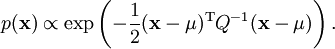
 means proportional; a pdf is always scaled so that its integral over the whole space is one. This
  , called the prior, was evolved in time by running the model and now is to be updated to account for new data. It is natural to assume that the error distribution of the data is known; data have to come with an error estimate, otherwise they are meaningless. Here, the data
  is assumed to have Gaussian pdf with covariance
  , where
  of the data
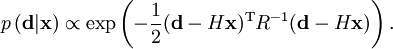
 instead of
  and the posterior pdf by
  . It can be shown by algebraic manipulations
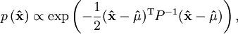
 and covariance
  given by the Kalman update formulas

![X=\left[ \mathbf{x}_{1},\ldots,\mathbf{x}_{N}\right] =\left[ \mathbf{x}_{i}\right].](images/math/e/9/1/e9120c2de8a8c4f6d57d6f06369ba34f.png)
 matrix whose columns are the ensemble members, and it is called the prior ensemble. Ideally, ensemble members would form a sample from the prior distribution. However, the ensemble members are not in general independent except in the initial ensemble, since every EnKF step ties them together. They are deemed to be approximately independent, and all calculations proceed as if they actually were independent.
 matrix
![D=\left[ \mathbf{d}_{1},\ldots,\mathbf{d}_{N}\right] =\left[ \mathbf{d}_{i}\right], \quad \mathbf{d}_{i}=\mathbf{d}+\epsilon_{i}, \quad \epsilon_{i} =N(0,R,)](images/math/9/f/5/9f5ae79aa1aa12178c62bd870027f058.png)
 consists of the data vector
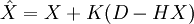
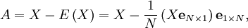
 denotes the matrix of all ones of the indicated size.

 and the inverse is replaced by a pseudoinverse, computed using the Singular Value Decomposition (SVD) .
 of the form

![\begin{align} \left[ HA\right] _{i} & =H\mathbf{x}_{i}-H\frac{1}{N}\sum_{j=1}^{N}\mathbf{x}_{j}\ & =h\left( \mathbf{x}_{i}\right) -\frac{1}{N}\sum_{j=1}^{N}h\left( \mathbf{x}_{j}\right) . \end{align}](images/math/c/6/1/c61c321463b102417eab7c81d2ad5230.png)
 with a fixed offset
  , which also does not need to be known explicitly. The above formula has been commonly used for a nonlinear observation function
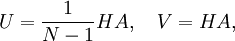
![\begin{align} P^{-1} & =\left( R+\frac{1}{N-1}HA\left( HA\right) ^{T}\right) ^{-1}\ & =R^{-1}\left[ I-\frac{1}{N-1}\left( HA\right) \left( I+\left( HA\right) ^{T}R^{-1}\frac{1}{N-1}\left( HA\right) \right) ^{-1}\left( HA\right) ^{T}R^{-1}\right] , \end{align}](images/math/2/3/e/23e2b59e059bb340e049077d158734ad.png)


