To use all functions of this page, please activate cookies in your browser.
My watch list
my.chemeurope.com
my.chemeurope.com
With an accout for my.chemeurope.com you can always see everything at a glance – and you can configure your own website and individual newsletter.
- My watch list
- My saved searches
- My saved topics
- My newsletter
Particle filter
They are usually used to estimate Bayesian models and are the sequential ('on-line') analogue of Markov chain Monte Carlo (MCMC) batch methods and are often similar to importance sampling methods. If well designed, particle filters can be much faster than MCMC. They are often an alternative to the Extended Kalman filter (EKF) or Unscented Kalman filter (UKF) with the advantage that, with sufficient samples, they approach the Bayesian optimal estimate, so they can be made more accurate than the EKF or UKF. The approaches can also be combined by using a version of the Kalman filter as a proposal distribution for the particle filter. Product highlight
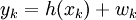
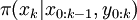
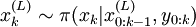
GoalThe particle filter aims to estimate the sequence of hidden parameters, xk for ModelParticle methods assume xk and the observations yk can be modeled in this form:
and with an initial distribution p(x0).
One example form of this scenario is where both vk and wk are mutually independent and identically distributed sequences with known probability density functions and Monte Carlo approximationParticle methods, like all sampling-based approaches (e.g., MCMC), generate a set of samples that approximate the filtering distribution and Generally, the algorithm is repeated iteratively for a specific number of k values (call this N).
Initializing xk = 0 | k = 0 for all particles provides a starting place to generate x1, which can then be used to generate x2, which can be used to generate x3 and so on up to k = N.
When done, the mean of xk over all the particles (or Sampling Importance Resampling (SIR)Sampling importance resampling (SIR) is a very commonly used
particle filtering algorithm, which approximates the filtering
distribution
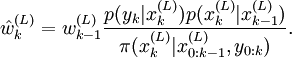
The importance weights SIR is a sequential (i.e., recursive) version of importance sampling.
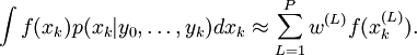
As in importance sampling, the expectation of a function
For a finite set of particles, the algorithm performance is dependent on the choice of the proposal distribution
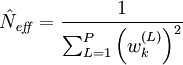
The optimal proposal distribution is given as the target distribution However, the transition prior is often used as importance function, since it is easier to draw particles (or samples) and perform subsequent importance weight calculations: Sampling Importance Resampling (SIR) filters with transition prior as importance function are commonly known as bootstrap filter and condensation algorithm. Resampling is used to avoid the problem of degeneracy of the algorithm, that is, avoiding the situation that all but one of the importance weights are close to zero. The performance of the algorithm can be also affected by proper choice of resampling method. The stratified resampling proposed by Kitagawa (1996) is optimal in terms of variance. A single step of sequential importance resampling is as follows:
Sequential Importance Sampling (SIS)
"Direct version" algorithmThe "direct version" algorithm is rather simple (compared to other particle filtering algorithms) and it uses composition and rejection.
To generate a single sample x at k from
The goal is to generate P "particles" at k using only the particles from k − 1. This requires that a Markov equation can be written (and computed) to generate a xk based only upon xk − 1. This algorithm uses composition of the P particles from k − 1 to generate a particle at k and repeats (steps 2-6) until P particles are generated at k. This can be more easily visualized if x is viewed as a two-dimensional array.
One dimension is k and the other dimensions is the particle number.
For example, x(k,L) would be the Lth particle at k and can also be written Other Particle Filters
See also
References
|
|
| This article is licensed under the GNU Free Documentation License. It uses material from the Wikipedia article "Particle_filter". A list of authors is available in Wikipedia. |


 , based only on the observed data
  . In contrast, the MCMC or importance sampling approach would model the full posterior
  .
.
 is a first order Markov process such that
 are conditionally independent provided that
 and
and  are known functions.
These two equations can be viewed as state space equations and look similar to the state space equations for the Kalman filter. If the functions
are known functions.
These two equations can be viewed as state space equations and look similar to the state space equations for the Kalman filter. If the functions 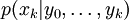 . So, with
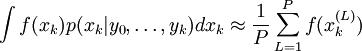
 ) is approximately the actual value of
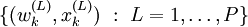
  by a weighted set
of particles
by a weighted set
of particles
 .
.
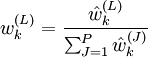
 are approximations to
the relative posterior probabilities (or densities) of the particles
such that
are approximations to
the relative posterior probabilities (or densities) of the particles
such that 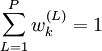 .
.
 .
.


 draw samples from the proposal distribution
 , then perform resampling:
 .
.
 :
:
 from its distribution
 using
using  where
where  (as done above in the algorithm).
Step 3 generates a potential
(as done above in the algorithm).
Step 3 generates a potential  ) at time

