To use all functions of this page, please activate cookies in your browser.
My watch list
my.chemeurope.com
my.chemeurope.com
With an accout for my.chemeurope.com you can always see everything at a glance – and you can configure your own website and individual newsletter.
- My watch list
- My saved searches
- My saved topics
- My newsletter
Fluorescence interference contrast microscopyFluorescence interference contrast (FLIC) microscopy is a microscopic technique developed to achieve z-resolution on the nanometer scale. FLIC occurs whenever fluorescent objects are in the vicinity of a reflecting surface (e.g. Si wafer). The resulting interference between the direct and the reflected light leads to a double sin2 modulation of the intensity, I, of a fluorescent object as a function of distance, h, above the reflecting surface. This allows for the nanometer height measurements. FLIC microscope is well suited to measuring the topography of a membrane that contains fluorescent probes e.g. an artificial lipid bilayer, or a living cell membrane or the structure of fluorescently labeled proteins on a surface. Product highlight
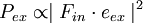
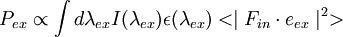
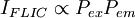
FLIC optical theoryGeneral two layer systemThe optical theory underlying FLIC was developed by Armin Lambacher and Peter Fromherz. They derived a relationship between the observed fluorescence intensity and the distance of the fluorophore from a reflective silicon surface. The observed fluorescence intensity, IFLIC, is the product of the excitation probability per unit time, Pex, and the probability of measuring an emitted photon per unit time, Pem. Both probabilities are a function of the fluorophore height above the silicon surface, so the observed intensity will also be a function of the fluorophore height. The simplest arrangement to consider is a fluorophore embedded in silicon dioxide (refractive index n1) a distance d from an interface with silicon (refractive index n0). The fluorophore is excited by light of wavelength λex and emits light of wavelength λem. The unit vector ''eex'' gives the orientation of the transition dipole of excitation of the fluorophore. Pex is proportional to the squared projection of the local electric field, Fin, which includes the effects of interference, on the direction of the transition dipole.
The squared projection Experimental SetupA silicon wafer is typically used as the reflective surface in a FLIC experiment. An oxide layer is then thermally grown on top of the silicon wafer to act as a spacer. On top of the oxide is placed the fluorescently labeled specimen, such as a lipid membrane, a cell or membrane bound proteins.
With the sample system built, all that is needed is an epifluorescence microscope and a CCD camera to make quantitative intensity measurements.
Analysis
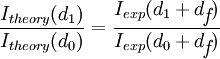
The basic analysis involves fitting the intensity data with the theoretical model allowing the distance of the fluorophore above the oxide surface (df) to be a free parameter.
The FLIC curves shift to the left as the distance of the fluorophore above the oxide increases. df is usually the parameter of interest, but several other free parameters are often included to optimize the fit. Normally an amplitude factor (a) and a constant additive term for the background (b) are included. The amplitude factor scales the relative model intensity and the constant background shifts the curve up or down to account for fluorescence coming from out of focus areas, such as the top side of a cell. Occasionally the numerical aperture (N.A.) of the microscope is allowed to be a free parameter in the fitting. The other parameters entering the optical theory, such as different indices of refraction, layer thicknesses and light wavelengths, are assumed constant with some uncertainty.
A FLIC chip may be made with oxide terraces of 9 or 16 different heights arranged in blocks. After a fluorescence image is captured, each 9 or 16 terrace block yields a separate FLIC curve that defines a unique df. The average df is found by compiling all the df values into a histogram.
References
|
|
| This article is licensed under the GNU Free Documentation License. It uses material from the Wikipedia article "Fluorescence_interference_contrast_microscopy". A list of authors is available in Wikipedia. |


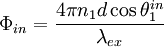
 is the angle of the incident light with respect to the silicon plane normal. Not only does interference modulate
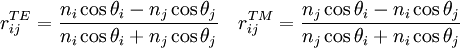
![F_{in} = \sin \gamma_{in} \left[\begin{array}{c}0 \\1 + r^{TE}_{10}\textit{e}^{ i\Phi_{in}} \\0\end{array}\right] + \cos \gamma _{in} \left[\begin{array}{c}\cos \theta ^{in}_{1}(1-r^{TM}_{10}\textit{e}^{i\Phi_{in}}) \\0 \\ \sin \theta ^{in}_{1}(1+r^{TM}_{10}\textit{e}^{i\Phi_{in}})\end{array}\right]](images/math/8/5/b/85b88d9398d8f7c28010704ab861d016.png)
![\textit{e}_{ex} = \left[\begin{array}{c}\cos \phi_{ex}\sin \theta_{ex}\\\sin \phi_{ex}\sin \theta_{ex} \\\cos \theta_{ex}\end{array}\right]](images/math/6/8/1/681aaa4e806014314090d5c5ae2a2b6c.png)
 must be averaged over these quantities to give the probability of excitation


Last viewed


