To use all functions of this page, please activate cookies in your browser.
My watch list
my.chemeurope.com
my.chemeurope.com
With an accout for my.chemeurope.com you can always see everything at a glance – and you can configure your own website and individual newsletter.
- My watch list
- My saved searches
- My saved topics
- My newsletter
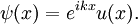
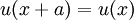
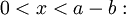
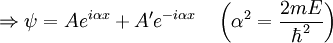
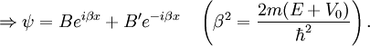
Particle in a one-dimensional lattice (periodic potential)In quantum mechanics, the particle in a one-dimensional lattice is a problem that occurs in the model of a periodic crystal lattice. The problem can be simplified from the 3D infinite potential barrier (particle in a box) to a one-dimensional case. The potential is caused by ions in the periodic structure of the crystal creating an electromagnetic field so electrons are subject to a regular potential inside the lattice. This is an extension of the free electron model that assumes zero potential inside the lattice. Product highlightProblem definitionWhen talking about solid materials, the discussion is mainly around crystals - periodic lattices. Here we will discuss a 1D lattice of positive ions. Assuming the spacing between two ions is a, the potential in the lattice will look something like this: The mathematical representation of the potential is a periodic function with a period a. According to Bloch's theorem, the wavefunction solution of the Schrödinger equation when the potential is periodic, can be written as: Where u(x) is a periodic function which satisfies: When nearing the edges of the lattice, there are problems with the boundary condition. Therefore, we can represent the ion lattice as a ring following the Born-von Karman boundary conditions. If L is the length of the lattice so that L >> a, then the number of ions in the lattice is so big, that when considering one ion, its surrounding is almost linear, and the wavefunction of the electron is unchanged. So now, instead of two boundary conditions we get one circular boundary condition: If N is the number of Ions in the lattice, then we have the relation: aN = L. Replacing in the boundary condition and applying Bloch's theorem will result in a quantization for k: Kronig-Penney modelIn order to simplify the problem the potential function is approximated by a rectangular potential: Using Bloch's theorem, we only need to find a solution for a single period, make sure it is continuous and smooth, and to make sure the function u(x) is also continuous and smooth.
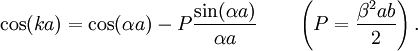
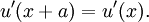
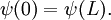
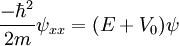
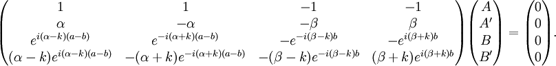
Considering a single period of the potential: In order to find u(x) in each region we need to manipulate the electron's wavefunction: And in the same manner: To complete the solution we need to make sure the probability function is continuous and smooth, i.e: And that u(x) and u'(x) are periodic These conditions yield the following matrix: In order for us not to have the trivial solution, the determinant of the matrix must be 0. This leads us to the following expression: In order to further simplify the expression, we will perform the following approximations: The expression will now be: See also
|
| This article is licensed under the GNU Free Documentation License. It uses material from the Wikipedia article "Particle_in_a_one-dimensional_lattice_(periodic_potential)". A list of authors is available in Wikipedia. |


![\cos(k a) = \cos(\beta b) \cos[\alpha(a-b)]-{\alpha^2+\beta^2 \over 2\alpha \beta} \sin(\beta b) \sin[\alpha(a-b)]. \,\!](images/math/b/c/3/bc31b9cb98b67eb26da14a720fa3f7db.png)