My watch list

Stimulated emission

In optics, stimulated emission is the process by which, when perturbed by a photon, matter may lose energy resulting in the creation of another photon. The perturbing photon is not destroyed in the process (cf. absorption), and the second photon is created with the same phase, frequency, polarization, and direction of travel as the original. Stimulated emission is really a quantum mechanical phenomenon but it can be understood in terms of a "classical" field and a quantum mechanical atom. The process can be thought of as "optical amplification" and it forms the basis of both the laser and maser.

Additional recommended knowledge

Don't let static charges disrupt your weighing accuracy

Better weighing performance in 6 easy steps

Overview

Electrons and how they interact with each other and electromagnetic fields form the basis for most of our understanding of chemistry and physics. Electrons have energy in proportion to how far they are on average from the nucleus of an atom; however quantum mechanical effects force electrons to take on quantized positions in orbitals. Thus, electrons are found in specific energy levels of an atom, as shown below:

The Pauli exclusion principle forces some electrons to be farther from the nucleus than others, which is why all the electrons in an atom do not simply occupy the 1s orbital. When electrons absorb energy either from light (photons) or from heat (phonons), they move farther away from the atomic nuclei but they are only allowed to absorb energy that will land them into specific energy levels. This leads to emission lines and absorption lines.

When an electron is excited, it will not stay that way forever. On average there is a lifetime for any particular energy level after which half of the electrons initially in that state will have decayed into a lower state. When such a decay occurs, the energy difference between the level the electron was at and the new level must be released either as a photon or a phonon. When an electron decays due to "timeout" it is said to be due to "spontaneous emission." The phase associated with the photon that is emitted is random and has to do with some quantum mechanical ideas concerning the atom's internal state. If a bunch of electrons were put into an excited state somehow and then left to relax, the resulting radiation would be very spectrally limited (only one wavelength of light would be present) but the individual photons would not be in phase with one another. This is also called fluorescence.

Other photons (i.e. an external electromagnetic field) will affect an atom's state. The quantum mechanical variables mentioned above are changed. Specifically the atom will act like a small electric dipole which will oscillate with the external field. One of the consequences of this oscillation is it encourages electrons to decay to the lower energy state. When it does this due to the presence of other photons, the released photon is in phase with the other photons and in the same direction as the other photons. This is known as stimulated emission.

Stimulated emission can be modelled mathematically by considering an atom which may be in one of two electronic energy states, the ground state (1) and the excited state (2), with energies E₁ and E₂ respectively.

If the atom is in the excited state, it may decay into the ground state by the process of spontaneous emission, releasing the difference in energies between the two states as a photon. The photon will have frequency ν and energy hν, given by:

E 2 - E 1 = h ν

where h is Planck's constant.

Alternatively, if the excited-state atom is perturbed by the electric field of a photon with frequency ν, it may release a second photon of the same frequency, in phase with the first photon. The atom will again decay into the ground state. This process is known as stimulated emission.

In a group of such atoms, if the number of atoms in the excited state is given by N, the rate at which stimulated emission occurs is given by:

$\frac{\partial N}{\partial t} = - B_{21} \rho (\nu) N$ ,

where B₂₁ is a proportionality constant for this particular transition in this particular atom (referred to as an Einstein B coefficient), and ρ(ν) is the radiation density of photons of frequency ν. The rate of emission is thus proportional to the number of atoms in the excited state, N, and the density of the perturbing photons.

The critical detail of stimulated emission is that the emitted photon is identical to the stimulating photon in that it has the same frequency, phase, polarization, and direction of propagation. The two photons, as a result, are totally coherent. It is this property that allows optical amplification to take place.

Although most directly related to the discussion of how lasers work, stimulated emission touches on some of the most basic concepts in physics and the interaction of light and matter. It is a very important topic, and key to the understanding of optics specifically and physics in general.

For various reasons, the frequencies of the various photons emitted will not be exactly the same. For example, since the individual atoms in a laser medium are typically at some finite temperature, the Doppler effect will cause the photon wavelengths to vary from atom to atom (although the actual mechanism involved is more complex because of the more complex relationship between relative wavelength of stimulating photon and emitted photon). The spectrum of the photons, then, will not be an infinitesimally thin line, but will be a distribution. This distribution in the spectrum of emitted photons is called "line shape".

Although there are many possible line shapes, it is common to model the spectral line shape function as a Lorentzian distribution:

$g(\nu) = {1 \over \pi } { (\Gamma / 2) \over (\nu - \nu_0)^2 + (\Gamma /2 )^2 }$

where

$\Gamma \,$ is the full width at half maximum, or FWHM, in hertz.

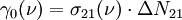
This model is generally valid as long as

$|\nu - \nu_0| << \nu_0 \,$

and

$\Gamma << \nu_0 \,$

The line shape function, regardless of the form that it takes, must satisfy the normalization condition of any probability distribution:

$\int_{-\infty}^{\infty} g(\nu) \cdot d \nu = 1$

which the Lorentzian satisfies.

The peak value of the Lorentzian line shape occurs at the line center:

$g(\nu = \nu_0) = {2 \over \pi \Gamma}$

It is also convenient to define the normalized line shape function:

$\bar{g}(\nu) = { g(\nu) \over g(\nu_0) } = { (\Gamma / 2)^2 \over (\nu - \nu_0)^2 + (\Gamma /2 )^2 }$

which is dimensionless, and which has a peak value, also at the line center, of

$\bar{g}(\nu = \nu_0) = 1$

Stimulated emission cross section

The stimulated emission cross section (in square meters) is

$\sigma_{21}(\nu) = A_{21} { \lambda^2 \over 8 \pi n^2} g(\nu)$

where

A₂₁ is the Einstein A coefficient (in radians per second),

λ is the wavelength (in meters),

n is the refractive index of the medium (dimensionless), and

g(ν) is the spectral line shape function (in seconds).

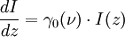
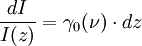
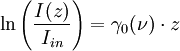
Optical amplification

Under certain conditions, stimulated emission can provide a physical mechanism for optical amplification. An external source of energy stimulates atoms in the ground state to transition to the excited state, creating what is called a population inversion. When light of the appropriate frequency passes through the inverted medium, the photons stimulate the excited atoms to emit additional photons of the same frequency, phase, and direction, resulting in an amplification of the input intensity.

The population inversion, in units of atoms per cubic meter, is

$\Delta N_{21} = \left( N_2 - {g_2 \over g_1} N_1 \right)$

where g₁ and g₂ are the degeneracies of energy levels 1 and 2, respectively.

Small signal gain equation

The intensity (in watts per square meter) of the stimulated emission is governed by the following differential equation:

${ dI \over dz} = \sigma_{21}(\nu) \cdot \Delta N_{21} \cdot I(z)$

as long as the intensity I(z) is small enough so that it does not have a significant effect on the magnitude of the population inversion. Grouping the first two factors together, this equation simplifies as

${ dI \over dz} = \gamma_0(\nu) \cdot I(z)$

where

$\gamma_0(\nu) = \sigma_{21}(\nu) \cdot \Delta N_{21}$

is the small-signal gain coefficient (in units of radians per meter). We can solve the differential equation using separation of variables:

${ dI \over I(z)} = \gamma_0(\nu) \cdot dz$

Integrating, we find:

$\ln \left( {I(z) \over I_{in}} \right) = \gamma_0(\nu) \cdot z$

$I(z) = I_{in}e^{\gamma_0(\nu) z}$

where

$I_{in} = I(z=0) \,$ is the optical intensity of the input signal (in watts per square meter).

Saturation intensity

The saturation intensity I_S is defined as the input intensity at which the gain of the optical amplifier drops to exactly half of the small-signal gain. We can compute the saturation intensity as

$I_S = {h \nu \over \sigma(\nu) \cdot \tau_S }$

where

h is Planck's constant, and

τ_S is the saturation time constant, which depends on the spontaneous emission lifetimes of the various transitions between the energy levels related to the amplification.

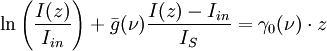
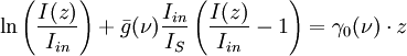
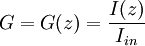
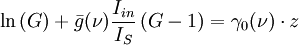
General gain equation

The general form of the gain equation, which applies regardless of the input intensity, derives from the general differential equation for the intensity I as a function of position z in the gain medium:

${ dI \over dz} = { \gamma_0(\nu) \over 1 + \bar{g}(\nu) { I(z) \over I_S } } \cdot I(z)$

where $I S$ is intensity. To solve, we first rearrange the equation in order to separate the variables, intensity I and position z:

${ dI \over I(z)} \left[ 1 + \bar{g}(\nu) { I(z) \over I_S } \right] = \gamma_0(\nu)\cdot dz$

Integrating both sides, we obtain

$\ln \left( { I(z) \over I_{in} } \right) + \bar{g}(\nu) { I(z) - I_{in} \over I_S} = \gamma_0(\nu) \cdot z$

$\ln \left( { I(z) \over I_{in} } \right) + \bar{g}(\nu) { I_{in} \over I_S } \left( { I(z) \over I_{in} } - 1 \right) = \gamma_0(\nu) \cdot z$

The gain G of the amplifier is defined as the optical intensity I at position z divided by the input intensity:

$G = G(z) = { I(z) \over I_{in} }$

Substituting this definition into the prior equation, we find the general gain equation:

$\ln \left( G \right) + \bar{g}(\nu) { I_{in} \over I_S } \left( G - 1 \right) = \gamma_0(\nu) \cdot z$

Small signal approximation

In the special case where the input signal is small compared to the saturation intensity, in other words,

$I_{in} << I_S \,$

then the general gain equation gives the small signal gain as

$\ln(G) = \ln(G_0) = \gamma_0(\nu) \cdot z$

$G = G_0 = e^{\gamma_0(\nu) z}$

which is identical to the small signal gain equation (see above).

Large signal asymptotic behavior

For large input signals, where

$I_{in} >> I_S \,$

the gain approaches unity

$G \rightarrow 1$

and the general gain equation approaches a linear asymptote:

$I(z) = I_{in} + { \gamma_0(\nu) \cdot z \over \bar{g}(\nu) } I_S$

References

Saleh, Bahaa E. A. and Teich, Malvin Carl (1991). Fundamentals of Photonics. New York: John Wiley & Sons. ISBN 0-471-83965-5.

Stimulated emission

Additional recommended knowledge

Don't let static charges disrupt your weighing accuracy

Better weighing performance in 6 easy steps

Essential Laboratory Skills Guide

Contents

Overview

Stimulated emission cross section

Optical amplification

Small signal gain equation

Saturation intensity

General gain equation

Small signal approximation

Large signal asymptotic behavior

References

See also

About chemeurope.com

About LUMITOS

Advertise with LUMITOS