Pipe Networks

Additional recommended knowledge

How to quickly check pipettes?

Correct Test Weight Handling Guide: 12 Practical Tips

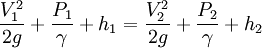
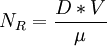
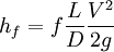
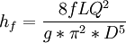
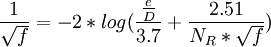
Daily Sensitivity Test

Pipe Networks generally refers to a common problem in Hydraulic Design.

In order to direct water to many individuals in a municipal water supply, many times the water is routed through a Water supply network. A major part of this network may consist of interconnected pipes. This network creates a special class of problems in hydraulic design typically referred to as pipe networks. The modern solution for this is to use specialized software such as WaterCad in order to automatically solve the problems. However, the problems can also be addressed with simpler methods like a spreadsheet equipped with a solver, or a modern graphing calculator.

Regardless of the computational platform, the problem itself consists primarily of two parts. Firstly, the Darcy-Weisbach formula is generally used to determine what is known as a friction factor. Some other equations that can be used are the Hazen-Williams equation (which is favored in the industry, but less accurate than the Darcy-Weisbach equation), and the Manning formula, which is more suited to calculation of open channel flow or culverts.

Regardless of which equation is used, the objective is to determine how much energy the water will lose by traveling through any pipe in the network. Bernoulli's principle is generally expressed in terms of energy per unit weight of water, or energy head. This is generally shown as

where V = Velocity, P is equal to pressure, and h is equal to elevation.

Essentially, as water flows through a pipe, friction will slow down the water in the pipe. If the velocity is fast enough, then the friction creates Turbulent flow. Water that is too slow for turbulence to be created is called Laminar flow. The Reynolds number determines what this will be. The equation is expressed:

where D is the diameter, V is the mean velocity, and mu is the kinematic viscosity of the fluid. In circular pipes, the critical Reynolds number is about 2000.

The most accurate expression showing the head loss due to friction in a pipe was derived by Henry Darcy(1803-1858) and Julius Weisbach(1806-1871).

Where f is the friction factor, L is the length of the pipe, D is the diameter, V is the velocity of the water, and g is the acceleration due to gravity.

When expressed in terms of Q for a circular pipe, the Darcy-Weisbach equation becomes:

So given this formulation, we can find out how much headloss to expect from a given pipe if we can determine what the friction factor will be. This is generally done by comparing the Reynolds number the Relative roughness of the pipe. The Roughness Height, e, is generally tabulated in terms of mm or ft for different materials. As an example, Cast iron might have a value of 0.26 mm, while rough concrete might be as high as 0.60 mm. The relative roughness is calculated by dividing the roughness height by the diameter of the pipe. e/D

One solution is to look up the friction factor graphically from a common graph called the Moody diagram. (L.F. Moody, "Friction factors for pipe flow," Trans. ASME, vol. 66, 1944.)

Moody Diagram: http://img95.imageshack.us/img95/1958/moodydr8.png

There is also an equation called the Colebrook equation that can be used, which was developed by C. F. Colebrook. It is cumbersome to use because it is implicit. The friction factor occurs on both sides of the expression. Given an initial guess value, usually two or three iterations are enough to give a good approximation with the following expression:

Once the friction factors are solved for, then we can start considering the network problem. We can solve the network by satisfying two conditions.

 1) At any junction, the flow into a junction equals the flow out of the junction.
 2) Between any two junctions, the head loss is independent of the path taken.

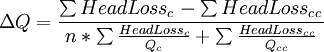
The classical approach for solving these networks is to use the Hardy Cross algorithm. In this formulation, first you go through and create guess values for the flows in the network. That is, if Q7 enters a junction and Q6 and Q4 leave the same junction, then the initial guess must satisfy Q7 = Q6 + Q4. After the initial guess is made, then, a loop is considered so that we can evaluate our second condition. Given a starting node, we work our way around the loop in a clockwise fashion, as illustrated by Loop 1. We add up the headlosses according to the Darcy-Weisbach equation for each pipe if Q is in the same direction as our loop like Q1, and subtract the headloss if the flow is in the reverse direction, like Q4. In order to satisfy the second condition, we should end up with 0 about the loop if the network is completely solved. If the actual sum of our headloss is not equal to 0, then we will adjust all the flows in the loop by an amount given by the following formula, where a positive adjustment is in the clockwise direction.

where n is 1.85 for Hazen-Williams or 2 for Darcy-Weisbach.

The clockwise specifier (c) means only the flows that are moving clockwise in our loop, while the counter-clockwise specifier (cc) is only the flows that are moving counter-clockwise.

This adjustment won't solve the problem, since with most networks we will have several loops. It is ok to do this adjustment, however, because our flow changes won't alter condition 1, and therefore, our other loops will still satisfy condition 1. However, we should use the results from the first loop if we progress to any other loops.

The more modern method is simply to create a set of conditions from your junctions and headloss criteria. Then, allow a solver in excel to adjust the Q values until it satisfies all the equations. The literal friction loss equations will use a term called Q², but we want to preserve any changes in direction. Create a separate equation for each loop where the headlosses are added up, but instead of squaring Q, use Abs(Q)*Q instead for the formulation so that any sign changes will reflect appropriately in the resulting headloss calculation.

References:

N. Hwang, R. Houghtalen, "Fundamentals of hydraulic Engineering Systems" Prentice Hall, Upper Saddle River, NJ. 1996.

L.F. Moody, "Friction factors for pipe flow," Trans. ASME, vol. 66, 1944.

C. F. Colebrook, "Turbulent flow in pipes, with particular reference to the transition region between smooth and rough pipe laws," Jour. Ist. Civil Engrs., London (Feb. 1939).