My watch list

Bose gas

An ideal Bose gas is a quantum-mechanical version of a classical ideal gas. It is composed of bosons, which have an integral value of spin, and obey Bose-Einstein statistics. The statistical mechanics of bosons were developed by Satyendra Nath Bose for photons, and extended to massive particles by Albert Einstein who realized that an ideal gas of bosons would form a condensate at a low enough temperature, unlike a classical ideal gas. This condensate is known as a Bose-Einstein condensate.

Additional recommended knowledge

What is the Correct Way to Check Repeatability in Balances?

How to ensure accurate weighing results every day?

Safe Weighing Range Ensures Accurate Results

1 The Thomas-Fermi approximation
2 Inclusion of the ground state
3 Thermodynamics
4 See also
5 References

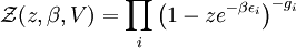
The Thomas-Fermi approximation

The thermodynamics of an ideal Bose gas is best calculated using the grand partition function. The grand partition function for a Bose gas is given by:

$\mathcal{Z}(z,\beta,V) = \prod_i \left(1-ze^{-\beta\epsilon_i}\right)^{-g_i}$

where each term in the product corresponds to a particular energy ε_i, g_i is the number of states with energy ε_i, z is the absolute activity, which may also be expressed in terms of the chemical potential μ by defining:

z (β,μ) = e βμ

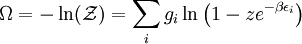
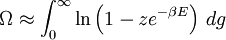
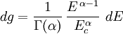
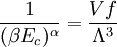
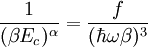
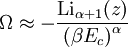
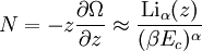
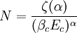
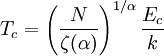
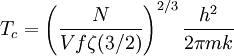
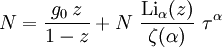
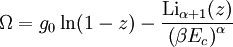
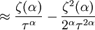
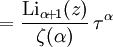
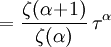
and β defined as:

$\beta = \frac{1}{kT}$

where k is Boltzmann's constant and T is the temperature. All thermodynamic quantities may be derived from the grand partition function and we will consider all thermodynamic quantities to be functions of only the three variables z , β (or T ), and V . All partial derivatives are taken with respect to one of these three variables while the other two are held constant. It is more convenient to deal with the dimensionless grand potential defined as:

$\Omega=-\ln(\mathcal{Z}) = \sum_i g_i \ln\left(1-ze^{-\beta\epsilon_i}\right)$

Following the procedure described in the gas in a box article, we can apply the Thomas-Fermi approximation which assumes that the average energy is large compared to the energy difference between levels so that the above sum may be replaced by an integral:

$\Omega\approx \int_0^\infty \ln\left(1-ze^{-\beta E}\right)\,dg$

The degeneracy dg may be expressed for many different situations by the general formula:

$dg = \frac{1}{\Gamma(\alpha)}\,\frac{E^{\,\alpha-1}}{ E_c^{\alpha}} ~dE$

where α is a constant, $E c$ is a "critical energy", and Γ is the Gamma function. For example, for a massive Bose gas in a box, α=3/2 and the critical energy is given by:

$\frac{1}{(\beta E_c)^\alpha}=\frac{Vf}{\Lambda^3}$

where Λ is the thermal wavelength. For a massive Bose gas in a harmonic trap we will have α=3 and the critical energy is given by:

$\frac{1}{(\beta E_c)^\alpha}=\frac{f}{(\hbar\omega\beta)^3}$

where V(r)=mω²r²/2 is the harmonic potential. It is seen that E_c is a function of volume only.

We can solve the equation for the grand potential by integrating the Taylor series of the integrand term by term, or by realizing that it is proportional to the Mellin transform of the Li₁(z exp(-β E)) where Li_s(x) is the polylogarithm function. The solution is:

$\Omega\approx-\frac{\textrm{Li}_{\alpha+1}(z)}{\left(\beta E_c\right)^\alpha}$

The problem with this continuum approximation for a Bose gas is that the ground state has been effectively ignored, giving a degeneracy of zero for zero energy. This inaccuracy becomes serious when dealing with the Bose-Einstein condensate and will be dealt with in the next section.

Inclusion of the ground state

The total number of particles is found from the grand potential by

$N = -z\frac{\partial\Omega}{\partial z} \approx\frac{\textrm{Li}_\alpha(z)}{(\beta E_c)^\alpha}$

The polylogarithm term must remain real and positive, and the maximum value it can possibly have is at z=1 where it is equal to ζ(α) where ζ is the Riemann zeta function. For a fixed N , the largest possible value that β can have is a critical value β_c where

$N = \frac{\zeta(\alpha)}{(\beta_c E_c)^\alpha}$

This corresponds to a critical temperature T_c=1/kβ_c below which the Thomas-Fermi approximation breaks down. The above equation can be solved for the critical temperature:

$T_c=\left(\frac{N}{\zeta(\alpha)}\right)^{1/\alpha}\frac{E_c}{k}$

For example, for $α = 3 / 2$ and using the above noted value of $E c$ yields

$T_c=\left(\frac{N}{Vf\zeta(3/2)}\right)^{2/3}\frac{h^2}{2\pi m k}$

Again, we are presently unable to calculate results below the critical temperature, because the particle numbers using the above equation become negative. The problem here is that the Thomas-Fermi approximation has set the degeneracy of the ground state to zero, which is wrong. There is no ground state to accept the condensate and so the equation breaks down. It turns out, however, that the above equation gives a rather accurate estimate of the number of particles in the excited states, and it is not a bad approximation to simply "tack on" a ground state term:

$N = N_0+\frac{\textrm{Li}_\alpha(z)}{(\beta E_c)^\alpha}$

where N₀ is the number of particles in the ground state condensate:

$N_0 = \frac{g_0\,z}{1-z}$

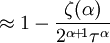
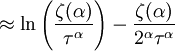
This equation can now be solved down to absolute zero in temperature. Figure 1 shows the results of the solution to this equation for α=3/2, with k=ε_c=1 which corresponds to a gas of bosons in a box. The solid black line is the fraction of excited states 1-N₀/N for N =10,000 and the dotted black line is the solution for N =1000. The blue lines are the fraction of condensed particles N₀/N The red lines plot values of the negative of the chemical potential μ and the green lines plot the corresponding values of z . The horizontal axis is the normalized temperature τ defined by

$\tau=\frac{T}{T_c}$

It can be seen that each of these parameters become linear in τ^α in the limit of low temperature and, except for the chemical potential, linear in 1/τ^α in the limit of high temperature. As the number of particles increases, the condensed and excited fractions tend towards a discontinuity at the critical temperature.

The equation for the number of particles can be written in terms of the normalized temperature as:

$N = \frac{g_0\,z}{1-z}+N~\frac{\textrm{Li}_\alpha(z)}{\zeta(\alpha)}~\tau^\alpha$

For a given N and τ, this equation can be solved for τ^α and then a series solution for z can be found by the method of inversion of series, either in powers of τ^α or as an asymptotic expansion in inverse powers of τ^α. From these expansions, we can find the behavior of the gas near T =0 and in the Maxwell-Boltzmann as T approaches infinity. In particular, we are interested in the limit as N approaches infinity, which can be easily determined from these expansions.

Thermodynamics

Adding the ground state to the equation for the particle number corresponds to adding the equivalent ground state term to the grand potential:

$\Omega = g_0\ln(1-z)-\frac{\textrm{Li}_{\alpha+1}(z)}{\left(\beta E_c\right)^\alpha}$

All thermodynamic properties may now be computed from the grand potential. The following table lists various thermodynamic quantities calculated in the limit of low temperature and high temperature, and in the limit of infinite particle number. An equal sign (=) indicates an exact result, while an approximation symbol indicates that only the first few terms of a series in $τ α$ is shown.

Quantity	General	$T \ll T_c\,$	$T \gg T_c\,$
z		$=1\,$	$\approx \frac{\zeta(\alpha)}{\tau^\alpha} -\frac{\zeta^2(\alpha)}{2^\alpha\tau^{2\alpha}}$
Vapor fraction $1-\frac{N_0}{N}\,$	$=\frac{\textrm{Li}_{\alpha}(z)}{\zeta(\alpha)} \,\tau^\alpha$	$=\tau^\alpha\,$	$=1\,$
Equation of state $\frac{PV\beta}{N}= -\frac{\Omega}{N}\,$	$= \frac{\textrm{Li}_{\alpha\!+\!1}(z)}{\zeta(\alpha)}\,\tau^\alpha$	$= \frac{\zeta(\alpha\!+\!1)}{\zeta(\alpha)}\,\tau^\alpha$	$\approx 1-\frac{\zeta(\alpha)}{2^{\alpha\!+\!1}\tau^\alpha}$
Gibbs Free Energy $G=\ln(z)\,$	$=\ln(z)\,$	$=0\,$	$\approx \ln\left(\frac{\zeta(\alpha)}{\tau^\alpha}\right) -\frac{\zeta(\alpha)}{2^{\alpha}\tau^\alpha}$

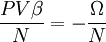
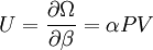
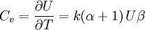
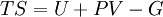
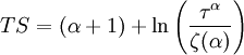
It is seen that all quantities approach the values for a classical ideal gas in the limit of large temperature. The above values can be used to calculate other thermodynamic quantities. For example, the relationship between internal energy and the product of pressure and volume is the same as that for a classical ideal gas over all temperatures:

$U=\frac{\partial \Omega}{\partial \beta}=\alpha PV$

A similar situation holds for the specific heat at constant volume

$C_v=\frac{\partial U}{\partial T}=k(\alpha+1)\,U\beta$

The entropy is given by:

$TS=U+PV-G\,$

Note that in the limit of high temperature, we have

$TS=(\alpha+1)+\ln\left(\frac{\tau^\alpha}{\zeta(\alpha)}\right)$

which, for α=3/2 is simply a restatement of the Sackur-Tetrode equation.

References

Huang, Kerson (1967). Statistical Mechanics. New York: John Wiley and Sons.
Isihara, A. (1971). Statistical Physics. New York: Academic Press.
Landau, L. D.; E. M. Lifshitz (1996). Statistical Physics, 3rd Edition Part 1. Oxford: Butterworth-Heinemann.
Pethick, C. J.; H. Smith (2004). Bose-Einstein Condensation in Dilute Gases. Cambridge: Cambridge University Press.
Yan, Zijun (2000). "General Thermal Wavelength and its Applications" (PDF). Eur. J. Phys 21: 625-631.

Categories: Gases | Thermodynamics | Statistical mechanics

This article is licensed under the GNU Free Documentation License. It uses material from the Wikipedia article "Bose_gas". A list of authors is available in Wikipedia.

Bose gas

Additional recommended knowledge

What is the Correct Way to Check Repeatability in Balances?

How to ensure accurate weighing results every day?

Safe Weighing Range Ensures Accurate Results

Contents

The Thomas-Fermi approximation

Inclusion of the ground state

Thermodynamics

See also

References

About chemeurope.com

About LUMITOS

Advertise with LUMITOS