To use all functions of this page, please activate cookies in your browser.
My watch list
my.chemeurope.com
my.chemeurope.com
With an accout for my.chemeurope.com you can always see everything at a glance – and you can configure your own website and individual newsletter.
- My watch list
- My saved searches
- My saved topics
- My newsletter
Bose–Einstein statistics
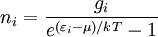
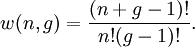
In statistical mechanics, Bose-Einstein statistics (or more colloquially B-E statistics) determines the statistical distribution of identical indistinguishable bosons over the energy states in thermal equilibrium. Fermi-Dirac and Bose-Einstein statistics apply when quantum effects have to be taken into account and the particles are considered "indistinguishable". The quantum effects appear if the concentration of particles (N/V) ≥ nq (where nq is the quantum concentration). The quantum concentration is when the interparticle distance is equal to the thermal de Broglie wavelength i.e. when the wavefunctions of the particles are touching but not overlapping. As the quantum concentration depends on temperature; high temperatures will put most systems in the classical limit unless they have a very high density e.g. a White dwarf. Fermi-Dirac statistics apply to fermions (particles that obey the Pauli exclusion principle), Bose-Einstein statistics apply to bosons. Both Fermi-Dirac and Bose-Einstein become Maxwell-Boltzmann statistics at high temperatures or low concentrations. Maxwell-Boltzmann statistics are often described as the statistics of "distinguishable" classical particles. In other words the configuration of particle A in state 1 and particle B in state 2 is different from the case where particle B is in state 1 and particle A is in state 2. When this idea is carried out fully, it yields the proper (Boltzmann) distribution of particles in the energy states, but yields non-physical results for the entropy, as embodied in Gibbs paradox. These problems disappear when it is realized that all particles are in fact indistinguishable. Both of these distributions approach the Maxwell-Boltzmann distribution in the limit of high temperature and low density, without the need for any ad hoc assumptions. Maxwell-Boltzmann statistics are particularly useful for studying gases. Fermi-Dirac statistics are most often used for the study of electrons in solids. As such, they form the basis of semiconductor device theory and electronics. Bosons, unlike fermions, are not subject to the Pauli exclusion principle: an unlimited number of particles may occupy the same state at the same time. This explains why, at low temperatures, bosons can behave very differently from fermions; all the particles will tend to congregate together at the same lowest-energy state, forming what is known as a Bose–Einstein condensate. B-E statistics was introduced for photons in 1920 by Bose and generalized to atoms by Einstein in 1924. The expected number of particles in an energy state i for B-E statistics is: with
This reduces to M-B statistics for energies ( εi − μ ) >> kT. Product highlight
HistoryIn the early 1920s Satyendra Nath Bose, a professor of University of Dhaka was intrigued by Einstein's theory of light waves being made of particles called photons. Bose was interested in deriving Planck's radiation formula, which Planck obtained largely by guessing. In 1900 Max Planck had derived his formula by manipulating the math to fit the empirical evidence. Using the particle picture of Einstein, Bose was able to derive the radiation formula by systematically developing a statistics of massless particles without the constraint of particle number conservation. Bose derived Planck's Law of Radiation by proposing different states for the photon. Instead of statistical independence of particles, Bose put particles into cells and described statistical independence of cells of phase space. Such systems allow two polarization states, and exhibit totally symmetric wavefunctions. He developed a statistical law governing the behaviour pattern of photons quite successfully. However, he was not able to publish his work; no journals in Europe would accept his paper, being unable to understand it. Bose sent his paper to Einstein, who saw the significance of it and used his influence to get it published. A derivation of the Bose–Einstein distributionSuppose we have a number of energy levels, labelled by index
Let With a little thought
(See Notes below)
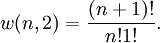
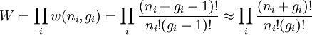
it can be seen that the number of ways of distributing
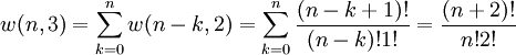
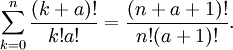
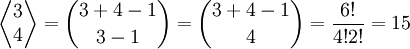
so that where we have used the following theorem involving binomial coefficients: Continuing this process, we can see that
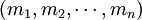
The number of ways that a set of occupation numbers
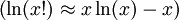
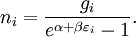
where the approximation assumes that Using the Taking the derivative with respect to
It can be shown thermodynamically that
It can also be shown that
Note that the above formula is sometimes written: where
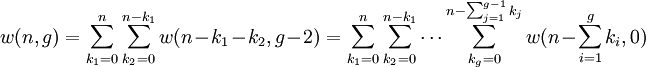
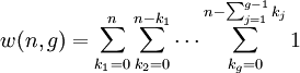
NotesThe purpose of these notes is to clarify some aspects of the derivation of the Bose-Einstein (B-E)
distribution for beginners. The enumeration of cases (or ways) in the B-E distribution can be recast as
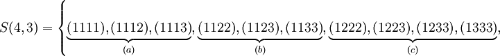
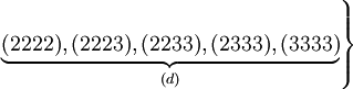
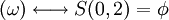
follows. Consider a game of dice throwing in which there are
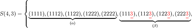
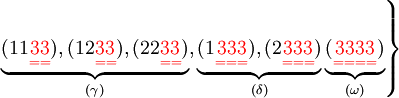
Then the quantity Example n=4, g=3:
Subset
Each element of
More generally, each element of
which is exactly the same as the
formula for
To understand the decomposition
or for example,
To this end, let's rearrange the elements of
Clearly, the subset
By deleting the index
In other words, there is a one-to-one correspondence between the subset
Similarly, it is easy to see that
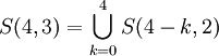
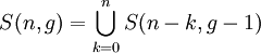
Thus we can write or more generally,
and since the sets are non-intersecting, we thus have
with the convention that
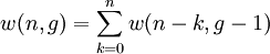
Continue the process, we arrive at the following formula Using the convention (7)2 above, we obtain the formula
keeping in mind that for
It can then be verified that (8) and (2) give the same result for
ReferencesAnnett, James F., "Superconductivity, Superfluids and Condensates", Oxford University Press, 2004, New York. Carter, Ashley H., "Classical ans Statistical Thermodynamics", Prentice-Hall, Inc., 2001, New Jersey. Griffiths, David J., "Introduction to Quantum Mechanics", 2nd ed. Pearson Education, Inc., 2005. See also
Categories: Statistical mechanics | Particle statistics |
|||||||||||||||||||||||||||
| This article is licensed under the GNU Free Documentation License. It uses material from the Wikipedia article "Bose–Einstein_statistics". A list of authors is available in Wikipedia. |
 and where:


 , each level
having energy
, each level
having energy  and containing a total of
 particles. Suppose each level contains
 distinct sublevels, all of which have the same energy, and which are distinguishable. For example, two particles may have different momenta, in which case they are distinguishable from each other, yet they can still have the same energy.
The value of
distinct sublevels, all of which have the same energy, and which are distinguishable. For example, two particles may have different momenta, in which case they are distinguishable from each other, yet they can still have the same energy.
The value of

 particles among the
 sublevels of an energy level. There is only one way of distributing
 . It is easy to see that
there are
. It is easy to see that
there are  ways of distributing

 .
Following the same procedure used in deriving the
.
Following the same procedure used in deriving the  is maximised, subject to the constraint that there be a fixed number of particles,
and a fixed energy. The maxima of
is maximised, subject to the constraint that there be a fixed number of particles,
and a fixed energy. The maxima of
 occur at the value of
 and, since it is easier to accomplish mathematically, we will maximise the
latter function instead. We constrain our solution using Lagrange multipliers forming the function:
and, since it is easier to accomplish mathematically, we will maximise the
latter function instead. We constrain our solution using Lagrange multipliers forming the function:

 gives
gives

 ,
where
,
where
 is
is  is the
  ,
where
,
where
 is the
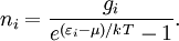
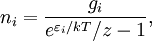
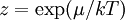 is the absolute activity.
 , for
, for  .
The constraints of the game is that the value of a dice
.
The constraints of the game is that the value of a dice
 , denoted by
 , in the previous throw, i.e.,
 . Thus a valid sequence of dice throws can be described by an
 , such that
  denote the set of these valid
 (there are
  elements in
  )
)
 is obtained by fixing all indices
 to
to
 , except for the last index,
 , which is incremented from
 .
Subset
.
Subset
 is obtained by fixing
 , and increment
 from
from
 to
to
 on the indices in
 must
automatically
take values in
must
automatically
take values in
 .
The construction of subsets
.
The construction of subsets
 and
and
 follows in the same manner.
 ;
the elements of such multiset are taken from the set
;
the elements of such multiset are taken from the set
 of cardinality


 of
of

 (shown in red with double underline)
in
the subset
(shown in red with double underline)
in
the subset
 of
of

 . We write


 (empty set)


 and
and
 being constants, we have

 ,
,
 ,
,
 , etc.
Last viewed


