To use all functions of this page, please activate cookies in your browser.
My watch list
my.chemeurope.com
my.chemeurope.com
With an accout for my.chemeurope.com you can always see everything at a glance – and you can configure your own website and individual newsletter.
- My watch list
- My saved searches
- My saved topics
- My newsletter
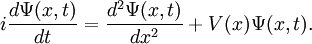
Diffusion Monte CarloDiffusion Monte Carlo (DMC) is a quantum Monte Carlo method that utilizes a Green function to solve the Schrödinger equation. DMC is potentially numerically exact, meaning that it can find the exact ground state energy within a given error for any quantum system. When actually attempting the calculation, one finds that for bosons, the algorithm is scales as a polynomial with the system size, but for fermions, DMC is exponentially scaling with the system size. This makes exact large-scale DMC simulations for fermions impossible; however, with a clever approximation known as fixed-node, very accurate results can be obtained. What follows is an explanation of the basic algorithm, how it works, why fermions cause a problem, and how the fixed-node approximation resolves this problem. The Projector MethodProduct highlightTo motivate the algorithm, let's look at the Schrödinger equation for a particle in some potential in one dimension:
We are usually interested in the wave function with the lowest energy eigenvalue, the ground state. We're going to write a slightly different version of the Schrödinger equation that will have the same energy eigenvalue, but, instead of being oscillatory, it will be convergent. Here it is:
Stochastic ImplementationNow we have an equation that, as we propagate it forward in time and adjust E0 appropriately, we find the
ground state of any given Hamiltonian. This is still a harder problem than classical mechanics, though, because instead of
propagating single positions of particles, we must propagate entire functions. In classical mechanics, we could simulate the
motion of the particles by setting x(t + τ) = x(t) + τv(t) + 0.5F(t)τ2, if we assume that the force is constant over the time span of τ. For the imaginary time Schrödinger equation, instead, we propagate forward in time using a convolution integral with a special function called a Green's function. So we get References
Categories: Quantum chemistry | Monte Carlo methods |
| This article is licensed under the GNU Free Documentation License. It uses material from the Wikipedia article "Diffusion_Monte_Carlo". A list of authors is available in Wikipedia. |


 We can condense the notation a bit by writing it in terms of an operator equation, with
 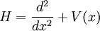 . So then we have
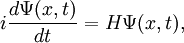 where we have to keep in mind that H is an operator, not a simple number or function. There are special functions, called eigenfunctions, for which
 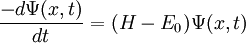 .
We've removed the imaginary number from the time derivative and added in a constant offset of
.
We've removed the imaginary number from the time derivative and added in a constant offset of 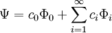 Since this is a linear differential equation, we can look at the action of each part separately. We already determined that
 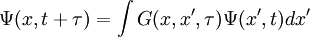 . Similarly to classical mechanics, we can only propagate for small slices of time; otherwise the Green's function is inaccurate. As the number of particles increases, the dimensionality of the integral increases as well, since we have to integrate over all coordinates of all particles. We can do these integrals by
 Last viewed


