My watch list
my.chemeurope.com  
Login  

Dissipative soliton


Dissipative solitons (DSs) are stable solitary localized structures that arise in nonlinear spatially extended dissipative systems due to mechanisms of self-organization. They can be considered as an extension of the classical soliton concept in conservative systems. An alternative terminology includes autosolitons, spots and pulses.

Apart from aspects similar to the behavior of classical particles like the formation of bound states, DSs exhibit entirely nonclassical behavior – e.g. scattering, generation and annihilation – all without the constraints of energy or momentum conservation. The excitation of internal degrees of freedom may result in a dynamically stabilized intrinsic speed, or periodic oscillations of the shape.

Contents

Historical development

Origin of the soliton concept

DSs have been experimentally observed for a long time. Helmholtz[1] measured the propagation velocity of nerve pulses in 1850. In 1902, Lehmann[2] found the formation of localized anode spots in long gas-discharge tubes. Nevertheless, the term "soliton" was originally developed in a different context. The starting point was the experimental detection of "solitary water waves" by Russell in 1834.[3] These observations initiated the theoretical work of Rayleigh[4] and Boussinesq[5] around 1870, which finally led to the approximate description of such waves by Korteweg and de Vries in 1895; that description is known today as the (conservative) KdV equation.[6]

On this background the term "soliton" was coined by Zabusky and Kruskal[7] in 1965. These authors investigated certain well localised solitary solutions of the KdV equation and named these objects solitons. Among other things they demonstrated that in 1-dimensional space solitons exist, e.g. in the form of two unidirectionally propagating pulses with different size and speed and exhibiting the remarkable property that number, shape and size are the same before and after collision.

Gardner at al.[8] introduced the inverse scattering technique for solving the KdV equation and proved that this equation is completely integrable. In 1972 Zakharov and Shabat[9] found another integrable equation and finally it turned out that the inverse scattering technique can be applied successfully to a whole class of equations (e.g. the nonlinear Schrödinger and Sine-Gordon equations). From 1965 up to about 1975, a common agreement was reached: to reserve the term soliton to pulse-like solitary solutions of conservative nonlinear partial differential equations that can be solved by using the inverse scattering technique.

Weakly and strongly dissipative systems

With increasing knowledge of classical solitons, possible technical applicability came into perspective, with the most promising one at present being the transmission of optical solitons via glass fibers for the purpose of data transmission. In contrast to systems with purely classical behavior, solitons in fibers dissipate energy and this cannot be neglected on an intermediate and long time scale. Nevertheless the concept of a classical soliton can still be used in the sense that on a short time scale dissipation of energy can be neglected. On an intermediate time scale one has to take small energy losses into account as a perturbation, and on a long scale the amplitude of the soliton will decay and finally vanish.[10]

There are however various types of systems which are capable of producing solitary structures and in which dissipation plays an essential role for their formation and stabilization. Although research on certain types of these DSs has been carried out for a long time (for example, see the research on nerve pulses culminating in the work of Hodgkin and Huxley[11] in 1952), since 1990 the amount of research has significantly increased (see e.g. [12][13]) Possible reasons are improved experimental devices and analytical techniques, as well as the availability of more powerful computers for numerical computations. Nowadays, it is common to use the term dissipative solitons for solitary structures in strongly dissipative systems.

Experimental observations of DSs

Today, DSs can be found in many different experimental set-ups. Examples include

  • Gas-discharge systems: plasmas confined in a discharge space which often has a lateral extension large compared to the main discharge length. DSs arise as current filaments between the electrodes and were found in DC systems with a high-ohmic barrier, [14] AC systems with a dielectric barrier,[15] and as anode spots,[16] as well as in an obstructed discharge with metallic electrodes.[17]


  • Semiconductor systems: these are similar to gas-discharges; however, instead of a gas, semiconductor material is sandwiched between two planar or spherical electrodes. Set-ups include Si and GaAs pin diodes,[18] n-GaAs,[19] and Si p+-n+-p-n-,[20] and ZnS:Mn structures.[21]
  • Nonlinear optical systems: a light beam of high intensity interacts with a nonlinear medium. Typically the medium reacts on rather slow time scales compared to the beam propagation time. Often, the output is fed back into the input system via single-mirror feedback or a feedback loop. DSs may arise as bright spots in a two-dimensional plane orthogonal to the beam propagation direction; one may, however, also exploit other effects like polarization. DSs have been observed for saturable absorbers,[22] degenerate optical parametric oscillators (DOPOs),[23] liquid crystal light valves (LCLVs),[24] alkali vapor systems,[25] photorefractive media,[26] and semiconductor microresonators.[27]
  • Chemical systems: realized either as one- and two-dimensional reactors or via catalytic surfaces, DSs appear as pulses (often as propagating pulses) of increased concentration or temperature. Typical reactions are the Belousov-Zhabotinsky_reaction,[28] the ferrocyanide-iodate-sulphite reaction as well as the oxidation of hydrogen,[29] CO,[30] or iron.[31] Nerve pulses[32] also belong to this class of systems.
  • Hydrodynamic systems: the most prominent realization of DSs are domains of convection rolls on a conducting background state in binary liquids.[36] Another example is a film dragging in a rotating cylindric pipe filled with oil.[37]
  • Electrical networks: large one- or two-dimensional arrays of coupled cells with a nonlinear current-voltage characteristic.[38] DSs are characterized by a locally increased current through the cells.

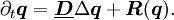
Remarkably enough, phenomenologically the dynamics of the DSs in many of the above systems are similar in spite of the microscopic differences. Typical observations are (intrinsic) propagation, scattering, formation of bound states and clusters, drift in gradients, interpenetration, generation, and annihilation, as well as higher instabilities.

Theoretical description of DSs

Most systems showing DSs are described by nonlinear partial differential equations. Discrete difference equations and cellular automata are also used. Up to now, modeling from first principles followed by a quantitative comparison of experiment and theory has been performed only rarely and sometimes also poses severe problems because of large discrepancies between microscopic and macroscopic time and space scales. Often simplified prototype models are investigated which reflect the essential physical processes in a larger class of experimental systems. Among these are
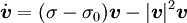
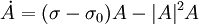
  • Reaction–diffusion systems, used for chemical systems, gas-discharges and semiconductors.[39] The evolution of the state vector q(xt) describing the concentration of the different reagents is determined by diffusion as well as local reactions:
\partial_t \boldsymbol{q} = \underline{\boldsymbol{D}} \Delta \boldsymbol{q} + \boldsymbol{R}(\boldsymbol{q}).
A frequently encountered example is the two-component Fitzhugh-Nagumo-type activator-inhibitor system
\left( \begin{array}{c} \tau_u \partial_t u\\\tau_v \partial_t v \end{array} \right) = \left(\begin{array}{cc} d_u^2 &0\\0&d_v^2 \end{array}\right) \left( \begin{array}{c} \Delta u\\ \Delta v \end{array} \right) + \left(\begin{array}{c} \lambda u -u^3 - \kappa_3 v +\kappa_1\\u-v \end{array}\right) .
Stationary DSs are generated by production of material in the center of the DSs, diffusive transport into the tails and depletion of material in the tails. A propagating pulse arises from production in the leading and depletion in the trailing end.[40] Among other effects, one finds periodic oscillations of DSs ("breathing"),[41][42] bound states,[43] and collisions, merging, generation and annihilation.[44]
  • Ginzburg-Landau type systems for a complex scalar q(xt) used to describe nonlinear optical systems, plasmas, Bose-Einstein condensation, liquid crystals and granular media.[45] A frequently found example is the cubic-quintic subcritical Ginzburg-Landau equation
\partial_t q = (d_r+ i d_i) \Delta q + l_r q + (c_r + i c_i)|q|^2 q + (q_r + i q_i) |q|^4 q.
An alternative formulation is given by considering the energy ρ = |q|2 for which one may derive the continuity equation
\partial_t \rho + \nabla \cdot \boldsymbol{m} = S = d_r (q \Delta q^{\ast} + q^{\ast} \Delta q) + 2 l_r \rho + 2 c_r \rho^2 + 2 q_r \rho^3 \quad\text{with} \quad\boldsymbol{m} = 2 d_i \text{Im}(q^{\ast}\nabla q).
One can thereby show that energy is produced in the flanks of the DSs and transported to the center and potentially to the tails where it is depleted. Dynamical phenomena include propagating DSs in 1d,[46] propagating clusters in 2d,[47] bound states and vortex solitons,[48] as well as "exploding DSs".[49]
  • The Swift-Hohenberg equation is used in nonlinear optics and in the granular media dynamics of flames or electroconvection. Swift-Hohenberg can be considered as an extension of the Ginzburg-Landau equation. It can be written as
\partial_t q = (s_r+ i s_i) \Delta^2 q + (d_r+ i d_i) \Delta q + l_r q + (c_r + i c_i)|q|^2 q + (q_r + i q_i) |q|^4 q.
For dr > 0 one essentially has the same mechanisms as in the Ginzburg-Landau equation.[50] For dr < 0, in the real Swift-Hohenberg equation one finds bistability between homogeneous states and Turing patterns. DSs are stationary localized Turing domains on the homogeneous background.[51] This also holds for the complex Swift-Hohenberg equations; however, propagating DSs as well as interaction phenomena are also possible, and observations include merging and interpenetration.[52]

Particle properties and universality

DSs in many different systems show universal particle-like properties. To understand and describe the latter, one may try to derive "particle equations" for slowly varying order parameters like position, velocity or amplitude of the DSs by adiabatically eliminating all fast variables in the field description. This technique is known from linear systems, however mathematical problems arise from the nonlinear models due to a coupling of fast and slow modes.[53]

Similar to low-dimensional dynamic systems, for supercritical bifurcations of stationary DSs one finds characteristic normal forms essentially depending on the symmetries of the system. E.g., for a transition from a symmetric stationary to an intrinsically propagating DS one finds the Pitchfork normal form

\dot{\boldsymbol{v}} = (\sigma - \sigma_0) \boldsymbol{v} - |\boldsymbol{v}|^2 \boldsymbol{v}

for the velocity v of the DS,[54] here σ represents the bifurcation parameter and σ0 the bifurcation point. For a bifurcation to a "breathing" DS, one finds the Hopf normal form

\dot{A} = (\sigma - \sigma_0) A - |A|^2 A

for the amplitude A of the oscillation.[42] In this way, a comparison between experiment and theory is facilitated.[55], [56] Note that the above problems do not arise for classical solitons as inverse scattering theory yields complete analytical solutions.

References

  1. ^ H. Helmholtz, Arch. Anat. Physiol. 57 (1850): 276
  2. ^ O. Lehmann, Ann. Phys. 4 (1902): 1
  3. ^ J. S. Russell, Report of the fourteenth meeting of the British Association for the Advancement of Science (1845): 311
  4. ^ J. W. Rayleigh, Phil. Mag. 1 (1876): 257
  5. ^ J. Boussinesq, Compt. Rend. Acad. Sc. 72 (1871): 755
  6. ^ D. J. Korteweg and H. de Vries, Phil. Mag. 39 (1895): 422
  7. ^ N. J. Zabusky and M. D. Kruskal, Phys. Rev. Lett. 15 (1965): 240
  8. ^ C. S. Gardner et al., Phys. Rev. Lett. 19 (1967): 1095
  9. ^ V. E. Zakharov and A. B. Shabat, Funct. Anal. Appl. 8 (1974): 226
  10. ^ Y. S. Kivshar and G. P. Agrawal, Optical Solitons. From Fibers to Photonic Crystals, Academic press (2003)
  11. ^ A. L. Hodgkin and A. F. Huxley, J. Physiol. 117 (1952): 500
  12. ^ B. S. Kerner and V. V. Osipov, Autosolitons. A New Approach to Problems of Self-Organization and Turbulence, Kluwer Academic Publishers (1995): 53
  13. ^ M. Bode and H.-G. Purwins, Physica D 86 (1995): 53
  14. ^ C. Radehaus et al., Phys. Lett. A 125 (1987): 92
  15. ^ I. Brauer et al., Phys. Rev. Lett. 84 (2000): 4104
  16. ^ S. M. Rubens and J. E. Henderson, Phys. Rev. 58 (1940): 446
  17. ^ S. Nasuno, Chaos 13 (2003): 1010
  18. ^ D. Jäger et al., Phys. Lett. A 117 (1986): 141
  19. ^ K. M. Mayer et al., Z. Phys. B 71 (1988): 171
  20. ^ F.-J. Niedernostheide et al., Phys. stat. sol. (b) 172 (1992): 249
  21. ^ M. Beale, Phil. Mag. B 68 (1993): 573
  22. ^ V. B. Tarananko et al., Phys. Rev. A 56 (1997): 1582
  23. ^ V. B. Tarananko et al., Phys. Rev. Lett. 81 (1998): 2236
  24. ^ A. Schreiber et al., Opt. Comm. 136 (1997): 415
  25. ^ B. Schäpers et al., Phys. Rev. Lett. 85 (2000): 748
  26. ^ C. Denz et al., Transverse-Pattern Formation in Photorefractive Optics, Springer Tracts in Modern Physics (2003): 188
  27. ^ S. Barland et al., Nature 419 (2002), 699
  28. ^ C. T. Hamik et al., J. Phys. Chem. A 105 (2001): 6144
  29. ^ S. L. Lane and D. Luss, Phys. Rev. Lett. 70 (1993): 830
  30. ^ H. H. Rotermund et al., Phys. Rev. Lett. 66 (1991): 3083
  31. ^ R. Suzuki, Adv. Biophys. 9 (1976): 115
  32. ^ A. L. Hodgkin and A. F. Huxley, J. Physiol. 117 (1952): 500
  33. ^ P. B. Umbanhowar et al., Nature 382 (1996): 793
  34. ^ O. Lioubashevski et al., Phys. Rev. Lett. 83 (1999): 3190
  35. ^ O. Lioubashevski et al., Phys. Rev. Lett. 76 (1996): 3959
  36. ^ G. Ahlers, Physica D 51 (1991): 421
  37. ^ F. Melo and S. Douady, Phys. Rev. Lett. 71 (1993): 3283
  38. ^ J. Nagumo et al., Proc. Inst. Radio Engin. Electr. 50 (1962): 2061
  39. ^ H.-G. Purwins et al., Dissipative Solitons in Reaction-Diffusion Systems, in Dissipative Solitons, Lecture Notes in Physics, Springer (2005)
  40. ^ E. Meron, Phys. Rep. 218 (1992):1
  41. ^ F.-J. Niedernostheide et al. in Nonlinearity with Disorder, Springer Proc. Phys. 67 (1992): 282
  42. ^ a b S. V. Gurevich et al., Phys. Rev. E 74 (2006), 066201
  43. ^ M. Or-Guil et al., Physica D 135 (2000): 154
  44. ^ C. P. Schenk et al., Phys. Rev. Lett. 78 (1997): 3781
  45. ^ I. S. Aranson and L. Kramer, Rev. Mod. Phys. 74 (2002): 99
  46. ^ V. V. Afanasjev et al., Phys. Rev. E 53 (1996): 1931
  47. ^ N. N. Rosanov et al., J. Exp. Theor. Phys. 102 (2006): 547
  48. ^ L.-C. Crasovan et al., Phys. Rev. E 63 (2000): 016605
  49. ^ J. M. Soto-Crespo et al., Phys. Rev. Lett. 85 (2000), 2937
  50. ^ J. M. Soto-Crespo and N. Akhmediev, Phys. Rev. E 66 (2002): 066610
  51. ^ H. Sakaguchi and H. R. Brandt,Physica D 97 (1996): 274
  52. ^ H. Sakaguchi and H. R. Brandt, Physica D 117 (1998): 95
  53. ^ R. Friedrich, Group Theoretic Methods in the Theory of Pattern Formation, in Collective dynamics of nonlinear and disordered systems, Springer (2004)
  54. ^ M. Bode, Physica D 106 (1997): 270
  55. ^ H. U. Bödeker et al., Phys. Rev. E 67 (2003): 056220
  56. ^ H. U. Bödeker et al., New J. Phys. 6 (2004): 62
 
This article is licensed under the GNU Free Documentation License. It uses material from the Wikipedia article "Dissipative_soliton". A list of authors is available in Wikipedia.
Your browser is not current. Microsoft Internet Explorer 6.0 does not support some functions on Chemie.DE